Lab: Community detection
Last update: 03 March, 2026
![]()
Modularity
1. Unipartite networks
We will start with finding communities in unipartite
networks. This is technically easier than in bipartite networks as the
implementations are straightforward in igraph. From the
help: “igraph implements a number of community detection
methods (see them below), all of which return an object of the class
communities. Because the community structure detection
algorithms are different, communities objects do not always
have the same structure.”
1.1 Undirected, unweighted
Let’s try to detect communities in the Chesapeake Food Web from the last lab. This is a quantitative food web but for simplicity at this first stage we will work with an undirected, unweighted graph.
Load the web:
chesapeake_nodes <- read.csv('data/Chesapeake_bay_nodes.csv', header=F)
names(chesapeake_nodes) <- c('nodeId','species_name')
chesapeake_links <- read.csv('data/Chesapeake_bay_links.csv', header=F)
names(chesapeake_links) <- c('from','to','weight')
ches_web <- graph.data.frame(chesapeake_links, vertices = chesapeake_nodes, directed = T)
Detect communities, note the as.undirected command:
ches_web_unweighted <- ches_web
ches_web_unweighted <- as.undirected(ches_web_unweighted)
E(ches_web_unweighted)$weight <- 1
cl <- cluster_louvain(ches_web_unweighted) # Can also use the weights = NULL argument
class(cl) # the result is of class communities
## [1] "communities"module_membership <- membership(cl)
cols <- data.frame(mem=unique(module_membership),
col= brewer.pal(length(unique(module_membership)), 'Set1'))
V(ches_web_unweighted)$module_membership <- module_membership
V(ches_web_unweighted)$color <- cols$col[match(V(ches_web_unweighted)$module_membership, cols$mem)]
plot(ches_web_unweighted, vertex.color=V(ches_web_unweighted)$color,
vertex.size=5, vertex.label=NA,
edge.arrow.width=0.3, edge.arrow.curve=0.5)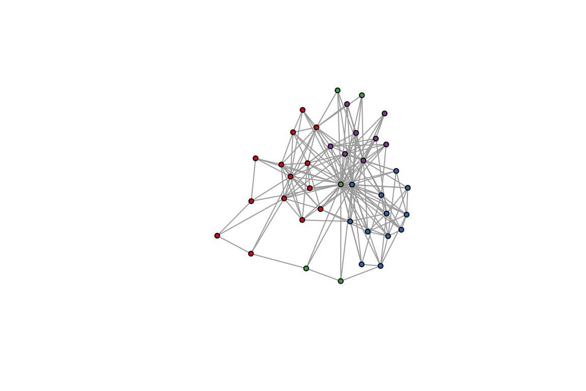
1. Identify the species in each module
2. Find modules in a different network.
3. Try a different community detection method,
like cluster_louvain. Are there any differences in module
assignments?
1.2 Undirected, weighted
We will use the same data set to see if there are any differences in the results.
#Notice the `weights` argument.
ches_web_undirected <- as.undirected(ches_web)
cl_wt <- cluster_louvain(ches_web_undirected, weights = E(ches_web_undirected)$weight)
class(cl_wt) # the result is of class communities
## [1] "communities"module_membership_wt <- membership(cl_wt)
cols <- data.frame(mem=unique(module_membership_wt),
col= brewer.pal(length(unique(module_membership_wt)), 'Set1'))
V(ches_web)$module_membership_wt <- module_membership_wt
V(ches_web)$color_wt <- cols$col[match(V(ches_web)$module_membership_wt, cols$mem)]
plot(as.undirected(ches_web), vertex.color=V(ches_web)$color_wt,
vertex.size=5, vertex.label=NA,
edge.arrow.width=0.3, edge.arrow.curve=0.5)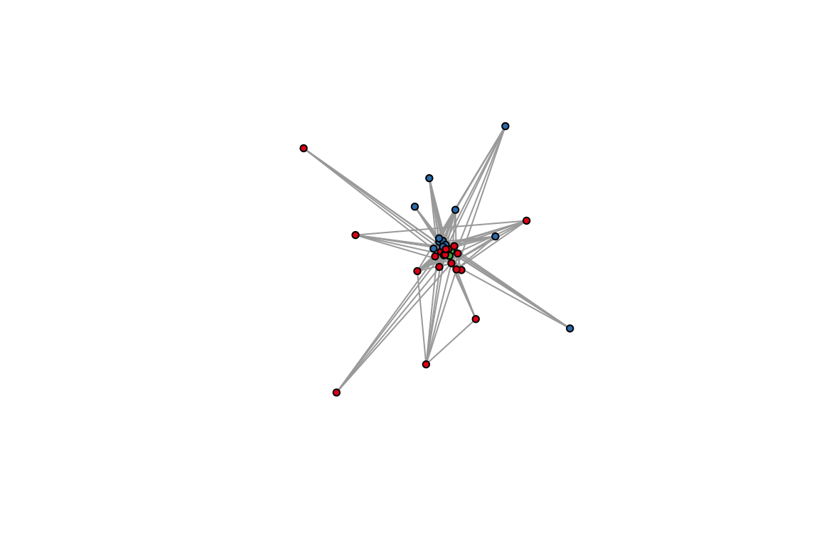 4. Compare the module assignments. How many nodes
were clustered with the same partners in both methods?
4. Compare the module assignments. How many nodes
were clustered with the same partners in both methods?
1.3 Directed networks
We will not touch upon directed networks in the context of modularity maximization, although there is a development for it by (Guimerà et al. 2007). The description of the sofware and the associated papers is in http://seeslab.info/downloads/bipartite-modularity/. The problem is that it is not available in an easy package, so you will have to hack your way through this.
2. Modularity in bipartite networks
The difference between bipartite and unipartite networks lies in the
“null” term of the modularity function, which should account for the
fact that edges cannot be expected between nodes of the same set. This
is well expalined in (Barber 2007) and (Guimerà et al.
2007) and reviewed in the context of ecology by (Thébault
2013). Each of these have their own software associated with
their papers. But for the sake of this exercise we are looking for an
implementation to optimize modularity maximization which will be readily
available, and also will allow us to analyze batches of networks (for
testing patterns against shuffled networks). The bipartite
package has a recent implementation of Stephen Beckett’s
DIRTLPAwb+ algorithm (Beckett 2016). This algorithm
maximizes a modularity function for weighted bipartite networks (Dormann et al.
2017), which is a recent extention of (Barber 2007)
method and is reduced to it if the input is a binary network. All this
can be a bit confusing so it is strongly suggested to read these papers
if you are about to apply these methods for community detection in your
research.
Note: this implementation is slow, and in my opinion not so much user friendly. But for Newmans’s modularity in bipartite networks it is the best I know of.
## [1] "originalWeb" "moduleWeb" "orderA" "orderB" "modules" "likelihood"## [1] 0.3044514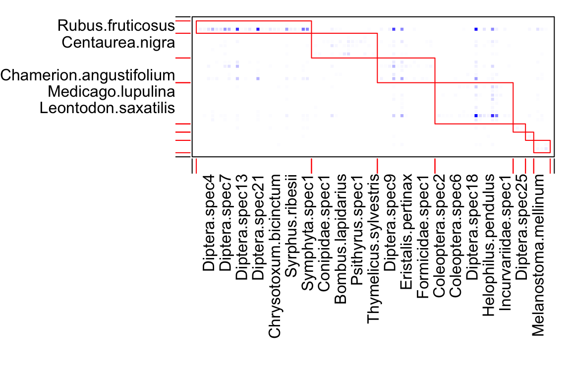
# let's look at the modules. The first element in the list is the whole network, so start with 2
module_list <- module_list[[2]]
for (i in 1:2){ # Show the two first modules.
  message(paste('Module:',i))
  print(module_list[[i]])
}
## [[1]]
## [1] "Rubus.fruticosus" "Daucus.carota"
##
## [[2]]
## [1] "Diptera.spec1" "Diptera.spec3" "Diptera.spec4" "Diptera.spec5"
## [5] "Diptera.spec6" "Scatophaga.stercoraria" "Diptera.spec7" "Diptera.spec8"
## [9] "Diptera.spec11" "Diptera.spec12" "Diptera.spec13" "Diptera.spec15"
## [13] "Diptera.spec19" "Diptera.spec20" "Diptera.spec21" "Tephretidae.spec1"
## [17] "Diptera.spec26" "Diptera.spec27" "Chrysotoxum.bicinctum" "Metasyrphus.corollae"
## [21] "Platycheirus.scutatus" "Syritta.pipiens" "Syrphus.ribesii" "Syrphus.vitripennis"
## [25] "Xanthogramma.pedissequum" "Parasitica" "Symphyta.spec1"## [[1]]
## [1] "Lotus.corniculatus" "Centaurea.nigra" "Knautia.arvensis" "Lathyrus.pratensis" "Trifolium.pratense"
##
## [[2]]
## [1] "Coleoptera.spec1" "Curculionidae.spec1" "Conipidae.spec1" "Diptera.spec16" "Eristalis.tenax"
## [6] "Rhingia.campestris" "Bombus.lapidarius" "Bombus.muscorum" "Bombus.pascuorum" "Bombus.terrestris"
## [11] "Psithyrus.spec1" "Apis.mellifera" "Polyommatus.icarus" "Maniola.jurtina" "Thymelicus.sylvestris"This list data structure is horrible for analysis. This code transforms it to a data frame:
# Transform the lists to data frames
m <- length(module_list) # Number of modules
mod_plants <- unlist(module_list, recursive = F)[seq(1,2*m,2)] # Assignments of plants
names(mod_plants) <- 1:m
mod_pollinators <- unlist(module_list, recursive = F)[seq(2,2*m,2)] # Assignments of pollinators
names(mod_pollinators) <- 1:m
tmp_plants <- data.frame(module = rep(names(mod_plants),
                                      sapply(mod_plants, length)),
                         species = unlist(mod_plants), type='Plants')
tmp_poillnators <- data.frame(module = rep(names(mod_pollinators),
                                           sapply(mod_pollinators, length)),
                              species = unlist(mod_pollinators), type='Pollinators')
# Make one data frame
module_assignments <- rbind(tmp_plants,tmp_poillnators)
5. Calculate modularity for the binary version of this web. How do the results differ?
6. Find another bipartite network in which you could hypothesize the existence of communities. Explain why this hypothesis is relevant for this data set. Analyze for communities. Do the results support the hypothesis (e.g., when you examine the nodes in each module).
7. Project the network and calculate modularity in each of the projections. Do the nodes that cluster together in the projection also cluster together in the bipartite version? Is there an difference in the interpretation between these two scenarios?
Flow modules with Infomap
3. Infomap
Modularity maximization is only one way to detect communities. While modularity is based on a null model, other methods are based on flow. The most popular is the Map Equation, originally developed by Martin Rosvall and Carl Bergstrom. Infomap, the implementation of the map equation, is the most flexible method available for community detection: it can handle unipartite, bipartite, and multilayer networks, weighted and directed. All the information you need is here: (http://www.mapequation.org/). To apply Infomap correctly you need to understand the mechanics and theory behind. This paper can help you: (Farage et al. 2021).
3.1 infomapecology R package
We will work with infomapecology and all the
documentations is here: https://ecological-complexity-lab.github.io/infomap_ecology_package/.
The package offers also a set of tools to convert data structures.
First, follow the instructions to install the package and infomap: https://ecological-complexity-lab.github.io/infomap_ecology_package/installation.
3.2 The monolayer class in infomapecology
infomapecology has a powerful way to convert between data structures.
For details run: ?create_monolayer_object. Here are two
basic examples.
Matrix to edge list: bipartite
data(memmott1999)
memmott1999_monolayer_object <- create_monolayer_network(memmott1999,
                                                        bipartite = T,
                                                        directed = F,
                                                        group_names = c('Pollinator','Plant'))
## [1] "Input: a bipartite matrix"## [1] "monolayer"## [1] "mode" "directed" "nodes" "mat" "edge_list" "igraph_object" "edge_list_ids"## # A tibble: 299 × 3
## from to weight
## <chr> <chr> <dbl>
## 1 Eriothrix.rufomaculata Agrimonium.eupatorium 1
## 2 Diptera.spec22 Agrimonium.eupatorium 1
## 3 Diptera.spec23 Agrimonium.eupatorium 1
## 4 Episyrphus.balteatus Agrimonium.eupatorium 2
## 5 Melanostoma.mellinum Agrimonium.eupatorium 1
## 6 Metasyrphus.corollae Agrimonium.eupatorium 1
## 7 Platycheirus.clypeatus Agrimonium.eupatorium 2
## 8 Sphaerophoria.scripta Agrimonium.eupatorium 2
## 9 Coleoptera.spec7 Leontodon.autumnalis 2
## 10 Diptera.spec10 Leontodon.autumnalis 1
## # ℹ 289 more rows## # A tibble: 104 × 3
## node_id node_group node_name
## <int> <chr> <chr>
## 1 1 Pollinator Coleoptera.spec1
## 2 2 Pollinator Coleoptera.spec2
## 3 3 Pollinator Coleoptera.spec3
## 4 4 Pollinator Coleoptera.spec4
## 5 5 Pollinator Coleoptera.spec5
## 6 6 Pollinator Coleoptera.spec6
## 7 7 Pollinator Coleoptera.spec7
## 8 8 Pollinator Cantharidae.spec1
## 9 9 Pollinator Curculionidae.spec1
## 10 10 Pollinator Diptera.spec1
## # ℹ 94 more rows## # A tibble: 299 × 3
## from to weight
## <chr> <chr> <dbl>
## 1 Eriothrix.rufomaculata Agrimonium.eupatorium 1
## 2 Diptera.spec22 Agrimonium.eupatorium 1
## 3 Diptera.spec23 Agrimonium.eupatorium 1
## 4 Episyrphus.balteatus Agrimonium.eupatorium 2
## 5 Melanostoma.mellinum Agrimonium.eupatorium 1
## 6 Metasyrphus.corollae Agrimonium.eupatorium 1
## 7 Platycheirus.clypeatus Agrimonium.eupatorium 2
## 8 Sphaerophoria.scripta Agrimonium.eupatorium 2
## 9 Coleoptera.spec7 Leontodon.autumnalis 2
## 10 Diptera.spec10 Leontodon.autumnalis 1
## # ℹ 289 more rowsEdge list with node attributes
We will use again the Otago food web.
Note that this is a slightly different version, with an edge list that has species names instead of ids.
## # A tibble: 6 × 41
##   node_name      node_id_original StageID SpeciesID Stage Species.StageID OrganismalGroup NodeType Resolution ResolutionNotes
##   <chr>                     <dbl>   <dbl>     <dbl> <chr>           <dbl> <chr>           <chr>    <chr>      <lgl>
## 1 Phytoplankton                 1       1         1 Adult             1.1 Plant           Common … Assemblage NA
## 2 Epipellic Flo…                2       1         2 Adult             2.1 Plant           Common … Assemblage NA
## 3 Macroalgae/Se…                3       1         3 Adult             3.1 Plant           Common … Assemblage NA
## 4 Zooplankton                   4       1         4 Adult             4.1 Zooplankton     Common … Assemblage NA
## 5 Meiofauna                     5       1         5 Adult             5.1 Meiofauna       Common … Assemblage NA
## 6 Bacteria                      6       1         6 Adult             6.1 Bacteria        Common … Assemblage NA
## # ℹ 31 more variables: Feeding <chr>, `Lifestyle(stage)` <chr>, `Lifestyle(species)` <chr>, `ConsumerStrategy(stage)` <chr>,
## #   System <lgl>, HabitatAffiliation <lgl>, Mobility <chr>, Residency <chr>, NativeStatus <lgl>, `BodySize(g)` <lgl>,
## #   BodySizeEstimation <lgl>, BodySizeNotes <lgl>, BodySizeN <lgl>, `Biomass(kg/ha)` <lgl>, BiomassEstimation <lgl>,
## #   BiomassNotes <lgl>, Kingdom <chr>, Phylum <chr>, Subphylum <lgl>, Superclass <lgl>, Class <chr>, Subclass <lgl>,
## #   Order <chr>, Suborder <lgl>, Infraorder <lgl>, Superfamily <lgl>, Family <chr>, Genus <chr>, SpecificEpithet <chr>,
## # Subspecies <lgl>, NodeNotes <lgl>## # A tibble: 1,206 × 3
## from to weight
## <chr> <chr> <dbl>
## 1 Phytoplankton Zooplankton 1
## 2 Zooplankton Zooplankton 1
## 3 Bacteria Zooplankton 1
## 4 Phytoplankton Meiofauna 1
## 5 Epipellic Flora Meiofauna 1
## 6 Macroalgae/Seagrass Meiofauna 1
## 7 Zooplankton Meiofauna 1
## 8 Meiofauna Meiofauna 1
## 9 Bacteria Meiofauna 1
## 10 Capitellid 1 Meiofauna 1
## # ℹ 1,196 more rowsnetwork_object <- create_monolayer_network(x=otago_links,
directed = T,
bipartite = F,
node_metadata = otago_nodes)## [1] "Input: an unipartite edge list"## # A tibble: 1,206 × 3
## from to weight
## <chr> <chr> <dbl>
## 1 Phytoplankton Zooplankton 1
## 2 Zooplankton Zooplankton 1
## 3 Bacteria Zooplankton 1
## 4 Phytoplankton Meiofauna 1
## 5 Epipellic Flora Meiofauna 1
## 6 Macroalgae/Seagrass Meiofauna 1
## 7 Zooplankton Meiofauna 1
## 8 Meiofauna Meiofauna 1
## 9 Bacteria Meiofauna 1
## 10 Capitellid 1 Meiofauna 1
## # ℹ 1,196 more rows## # A tibble: 140 × 42
## node_id node_name node_id_original StageID SpeciesID Stage Species.StageID OrganismalGroup NodeType Resolution
## <int> <chr> <dbl> <dbl> <dbl> <chr> <dbl> <chr> <chr> <chr>
## 1 1 Phytoplankton 1 1 1 Adult 1.1 Plant Common … Assemblage
## 2 2 Epipellic Flora 2 1 2 Adult 2.1 Plant Common … Assemblage
## 3 3 Macroalgae/Seagrass 3 1 3 Adult 3.1 Plant Common … Assemblage
## 4 4 Zooplankton 4 1 4 Adult 4.1 Zooplankton Common … Assemblage
## 5 5 Meiofauna 5 1 5 Adult 5.1 Meiofauna Common … Assemblage
## 6 6 Bacteria 6 1 6 Adult 6.1 Bacteria Common … Assemblage
## 7 7 Anthopleura aureorad… 7 1 7 Adult 7.1 Anthozoan Taxon Species
## 8 8 Edwardsia sp. 8 1 8 Adult 8.1 Anthozoan Taxon Species
## 9 9 Enopla 1 9 1 9 Adult 9.1 Nemertean Taxon Species
## 10 10 Enopla 2 10 1 10 Adult 10.1 Nemertean Taxon Species
## # ℹ 130 more rows
## # ℹ 32 more variables: ResolutionNotes <lgl>, Feeding <chr>, `Lifestyle(stage)` <chr>, `Lifestyle(species)` <chr>,
## # `ConsumerStrategy(stage)` <chr>, System <lgl>, HabitatAffiliation <lgl>, Mobility <chr>, Residency <chr>,
## # NativeStatus <lgl>, `BodySize(g)` <lgl>, BodySizeEstimation <lgl>, BodySizeNotes <lgl>, BodySizeN <lgl>,
## # `Biomass(kg/ha)` <lgl>, BiomassEstimation <lgl>, BiomassNotes <lgl>, Kingdom <chr>, Phylum <chr>, Subphylum <lgl>,
## # Superclass <lgl>, Class <chr>, Subclass <lgl>, Order <chr>, Suborder <lgl>, Infraorder <lgl>, Superfamily <lgl>,
## # Family <chr>, Genus <chr>, SpecificEpithet <chr>, Subspecies <lgl>, NodeNotes <lgl>## Phytoplankton Epipellic Flora Macroalgae/Seagrass Zooplankton Meiofauna
## Phytoplankton 0 0 0 0 0
## Epipellic Flora 0 0 0 0 0
## Macroalgae/Seagrass 0 0 0 0 0
## Zooplankton 1 0 0 1 0
## Meiofauna 1 1 1 1 13.3 Running Infomap
The general work flow is to create a monolayer object, run infomap
and parse the results. The function run_infomap_monolayer
has many options—make sure you read the help. It can also accept
specific flags for Infomap (details in mapequation.org) via the
....
Note that the flow model must match your question and data. Details in the SI of our paper: https://besjournals.onlinelibrary.wiley.com/doi/10.1111/2041-210X.13569 (Farage et al. 2021).
infomap_object <- run_infomap_monolayer(memmott1999_monolayer_object,
                                        infomap_executable='./Infomap',
                                        flow_model = 'undirected',
                                        silent=T, trials=20, two_level=T, seed=123, ...='--ftree')
## [1] "Creating a link list..."
## running: ././Infomap infomap.txt . --tree --seed 123 -N 20 -f undirected --silent --two-level --ftree
## [1] "Removing auxilary files..."## [1] "/Users/shai/GitHub/ecomplab/network_course/website_source"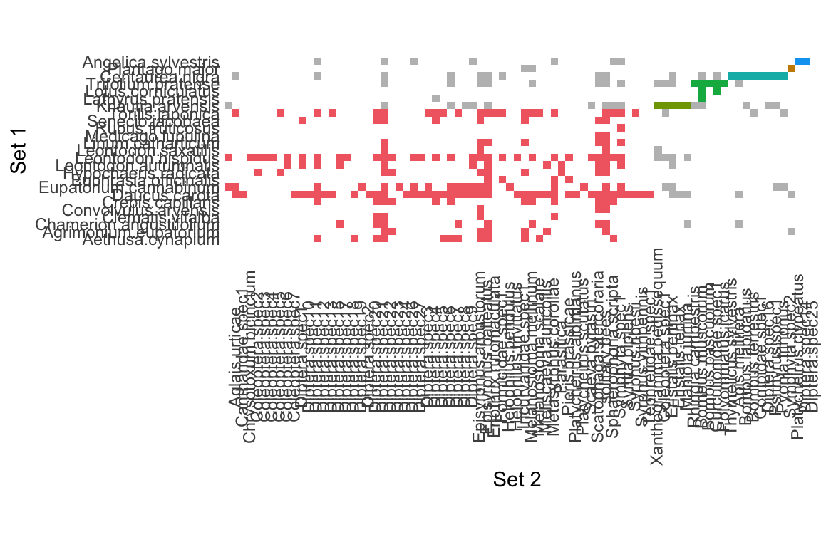
## [1] "infomap_monolayer"3.4 Exploring the modules
The infomap_monolayer object contains all the necessary
information for downstream analysis.
## [1] "call" "L" "m" "modules" "edge_list" "L_sim" "m_sim" "pvalue"## [1] 4.56751## [1] 6## # A tibble: 104 × 7
## node_id node_name flow levels module_level1 module_level2 node_group
## <dbl> <chr> <dbl> <dbl> <dbl> <dbl> <chr>
## 1 1 Coleoptera.spec1 0.000916 1 2 5 Pollinator
## 2 2 Coleoptera.spec2 0.000916 1 1 50 Pollinator
## 3 3 Coleoptera.spec3 0.000458 1 1 64 Pollinator
## 4 4 Coleoptera.spec4 0.000229 1 1 75 Pollinator
## 5 5 Coleoptera.spec5 0.000229 1 1 74 Pollinator
## 6 6 Coleoptera.spec6 0.000687 1 1 59 Pollinator
## 7 7 Coleoptera.spec7 0.000916 1 1 58 Pollinator
## 8 8 Cantharidae.spec1 0.00229 1 1 37 Pollinator
## 9 9 Curculionidae.spec1 0.000458 1 3 5 Pollinator
## 10 10 Diptera.spec1 0.00115 1 1 49 Pollinator
## # ℹ 94 more rows# Number of species in modules:
infomap_object$modules %>%
group_by(module_level1) %>%
summarise(module_size=n_distinct(node_name))## # A tibble: 6 × 2
## module_level1 module_size
## <dbl> <int>
## 1 1 76
## 2 2 6
## 3 3 8
## 4 4 9
## 5 5 2
## 6 6 38. Explore the modules. For example, how many
plants and pollinators in each module? You will need to link the module
assignments from the infomap_monolayer object and the nodes
from the monolayer object.
Stochastic Block Models
4. Stochastic Block Models (SBMs)
SBMs are a probabilistic approach to detecting communities in networks. They assume that nodes are partitioned into communities, and the probability of an edge between any two nodes depends on their community memberships.
In this section, we will use the blockmodels package to
fit an SBM to the memmott1999 plant-pollinator network. This method will
help us identify the underlying community structure based on edge
probabilities.
First, ensure you have the blockmodels package installed
and loaded:
if (!requireNamespace("blockmodels", quietly = TRUE)) {
  install.packages("blockmodels")
}
library(blockmodels)

# transforming to unweighted network
memmott1999_binary <- 1*(memmott1999>0)
# Fit an SBM using the variational method. Note we are using a bipartite network, hence the "LBM"
sbm_fit <- BM_bernoulli("LBM", memmott1999_binary)
sbm_fit$plotting <- '' # Set plots of the convergence process to off
sbm_fit$verbosity <- 0 # No output (you should not use this, it is for making this file readable)
sbm_fit$estimate()
# Select the best number of clusters (based on maximum likelihood)
best_run = which.max(sbm_fit$ICL)
# Extract the community memberships
community_assignments <- sbm_fit$memberships[[best_run]]
community_assignments$plot() # Left plot plants, right plot pollinators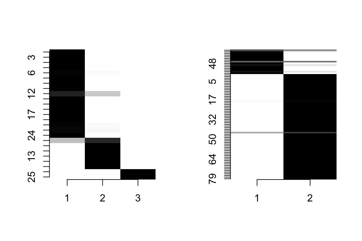
groups_P <- community_assignments$Z1 # Groups of plants (rows plants, columns are pollinators)
groups_A <- community_assignments$Z2 # Groups of pollinators (rows plants, columns are pollinators)
group_id_P <- apply(groups_P, 1, FUN = which.max) # The node belongs to a cluster to which it has highest probability
group_id_A <- apply(groups_A, 1, FUN = which.max) # The node belongs to a cluster to which it has highest probability
groups_P <- tibble(node=rownames(memmott1999), group=group_id_P) %>% mutate(type='plant')
groups_A <- tibble(node=colnames(memmott1999), group=group_id_A) %>% mutate(type='pollinator')
results <- bind_rows(groups_P, groups_A)
The ‘pi’ parameter represents the probability that an edge exists between a node in block \(a\) and a node in block \(b\), thereby characterizing the network’s block-level connectivity structure.
# pi parameter
pi <- as.data.frame(sbm_fit$model_parameters[[best_run]]$pi) %>%
  rownames_to_column("group_1") %>%
  gather("group_2", "pi", starts_with("V"))

# plotting
pi %>%
  ggplot(aes(x = group_2, y = group_1, fill = pi, label=round(pi,3))) +
  geom_tile() +
  geom_text()+
  theme_classic()+
  scale_fill_distiller(palette = "Blues", direction = 1) +
theme(axis.text = element_text(size = 10, color = 'black'), title = element_text(size = 14)) +
  labs(x="Pollinators Group", y="Plants Group")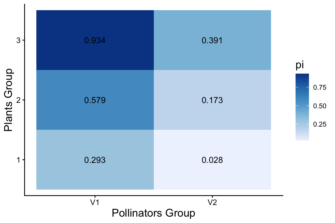
9. Use igraph to plot the network with nodes colored by group id.
10. Compare the SBM community assignments with those obtained from Infomap. What are the similarities and differences in the detected modules?
11. Select another data set and run SBM analysis.