#devtools::install_github("manlius/muxViz")
# library(muxViz)
library(emln)
library(infomapecology)
library(igraph)
library(bipartite)
library(tidyverse)
library(magrittr)
library(readxl)
library(ggalluvial)
library(ggplot2)
library(tidyr)
library(dplyr)
library(purrr)
library(network)
library(ggnetwork)

In this exercise we will rely heavily on the EMLN package. See the full description and code in https://ecological-complexity-lab.github.io/emln_package/.

Code

Download R code

1. Data structures: Monolayer networks

To understand multilayer network data structures we must first understand the monolayer data structures. We did this in our first exercise. Therefore, we assume you already know this!

The EMLN package has built in functions to convert between edge lists and matrices. You should follow the code here and make sure you understand it before delvoing into multilayer networks.

2. Data structures: Multilayer networks

We will again largely follow the guide of the EMLN package here. But before we do, let’s learn the data structures.

Multilayer network components

We can divide multilayer networks into those with and without interlayer edges:

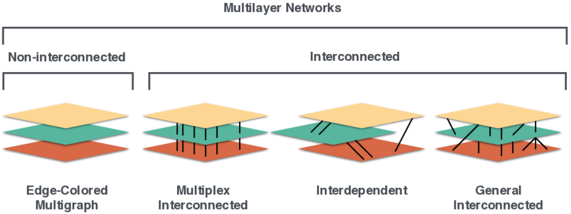
And having the following components:

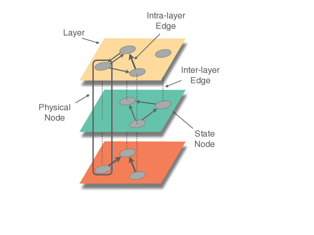
(Figures copy-righted to Manlio de Domenico, https://github.com/manlius/muxViz/blob/master/gui-old/theory/README.md)

Three representations of a multilayer network

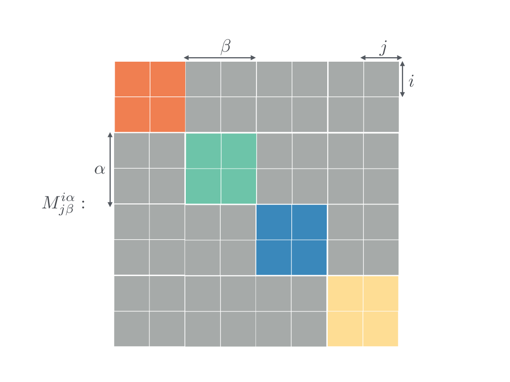
We can represent a multilayer using a graph, an extended edge list or a tensor (matrix with more than 2 dimensions). Tensors can be flattened to supra-adjacency matrices. This can be seen in the middle panel.

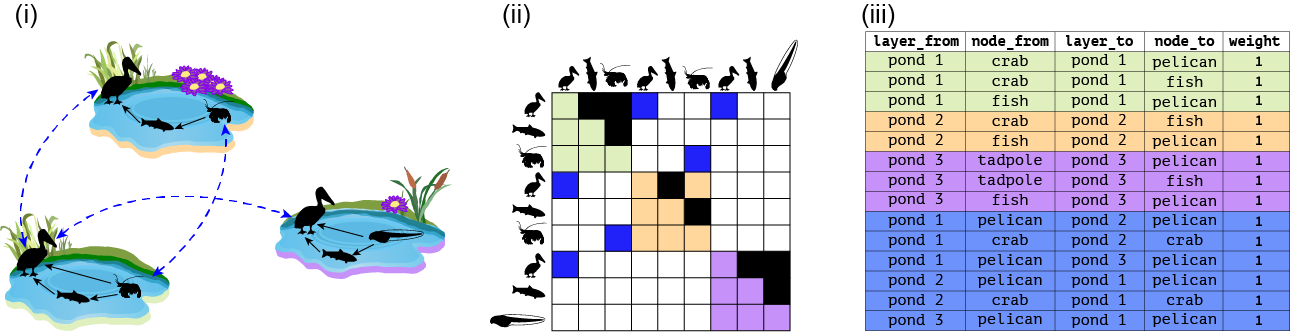
And here:

Figure copy-righted to Manlio de Domenico, https://github.com/manlius/muxViz/blob/master/gui-old/theory/README.md

No interlayer links.

Now that we understand structures, let’s see how to encode them.

Toy example

This is the easiest case of disconnected layers. Here is the pond example without interlayer links:

pond_1 <- matrix(c(0,1,1,0,0,1,0,0,0), byrow = T, nrow = 3, ncol = 3, dimnames = list(c('pelican','fish','crab'),c('pelican','fish','crab')))

pond_2 <- matrix(c(0,1,0,0,0,1,0,0,0), byrow = T, nrow = 3, ncol = 3, dimnames = list(c('pelican','fish','crab'),c('pelican','fish','crab')))

pond_3 <- matrix(c(0,1,1,0,0,1,0,0,0), byrow = T, nrow = 3, ncol = 3, dimnames = list(c('pelican','fish','tadpole'),c('pelican','fish','tadpole')))

layer_attrib <- tibble(layer_id=1:3,
                     layer_name=c('pond_1','pond_2','pond_3'),
                     location=c('valley','mid-elevation','uphill'))

multilayer <- create_multilayer_network(list_of_layers = list(pond_1, pond_2, pond_3), 
                                        bipartite = F, 
                                        directed = T)

## [1] "Layer attributes not provided, I added them (see layer_attributes in the final object)"
## [1] "Layer #1 processing."
## [1] "Done."
## [1] "Layer #2 processing."
## [1] "Done."
## [1] "Layer #3 processing."
## [1] "Done."
## [1] "Creating extended link list with node IDs"
## [1] "Organizing state nodes"

multilayer$extended

## # A tibble: 8 × 5
##   layer_from node_from layer_to node_to weight
##   <chr>      <chr>     <chr>    <chr>    <dbl>
## 1 layer_1    fish      layer_1  pelican      1
## 2 layer_1    crab      layer_1  pelican      1
## 3 layer_1    crab      layer_1  fish         1
## 4 layer_2    fish      layer_2  pelican      1
## 5 layer_2    crab      layer_2  fish         1
## 6 layer_3    fish      layer_3  pelican      1
## 7 layer_3    tadpole   layer_3  pelican      1
## 8 layer_3    tadpole   layer_3  fish         1

The multilayer class

Go over the resulting multilayer class and see what it includes.

Real data

Let’s take an example with real data, using the data of Kefi et al 2016. This is a node-aligned multiplex network with three layers: trophic interactions, non-trophic positive interactions and non-trophic negative interactions. First, we will see how we can use matrices as input. Along the way we perform sanity checks such as making sure the number and identity of of species is the same in the 3 layers.

# Load and organize the trophic interactions matrix
chilean_TI <- read_delim('data/chilean_TI.txt', delim = '\t')
nodes <- chilean_TI[,2]
names(nodes) <- 'Species'
chilean_TI <- data.matrix(chilean_TI[,3:ncol(chilean_TI)])
dim(chilean_TI)

## [1] 106 106

dimnames(chilean_TI) <- list(nodes$Species,nodes$Species)

# Load and organize the negative non-trophic interactions matrix
chilean_NTIneg <- read_delim('data/chilean_NTIneg.txt', delim = '\t')
nodes <- chilean_NTIneg[,2]
names(nodes) <- 'Species'
chilean_NTIneg <- data.matrix(chilean_NTIneg[,3:ncol(chilean_NTIneg)])
dim(chilean_NTIneg)

## [1] 106 106

dimnames(chilean_NTIneg) <- list(nodes$Species,nodes$Species)

# Are all row and column names the same?
setequal(rownames(chilean_TI), rownames(chilean_NTIneg))

## [1] TRUE

setequal(colnames(chilean_TI), colnames(chilean_NTIneg))

## [1] TRUE

chilean_NTIneg <- chilean_NTIneg[rownames(chilean_TI),colnames(chilean_TI)]
all(rownames(chilean_TI)==rownames(chilean_NTIneg))

## [1] TRUE

# Load and organize the negative non-trophic positive matrix
chilean_NTIpos <- read_delim('data/chilean_NTIpos.txt', delim = '\t')
nodes <- chilean_NTIpos[,2]
names(nodes) <- 'Species'
chilean_NTIpos <- data.matrix(chilean_NTIpos[,3:ncol(chilean_NTIpos)])
dim(chilean_NTIpos)

## [1] 106 106

dimnames(chilean_NTIpos) <- list(nodes$Species,nodes$Species)

# Are all row and column names the same?
setequal(rownames(chilean_TI), rownames(chilean_NTIpos))

## [1] TRUE

setequal(colnames(chilean_TI), colnames(chilean_NTIpos))

## [1] TRUE

chilean_NTIpos <- chilean_NTIpos[rownames(chilean_TI),colnames(chilean_TI)]
all(rownames(chilean_TI)==rownames(chilean_NTIpos))

## [1] TRUE

# Total number of links
sum(chilean_TI, chilean_NTIpos, chilean_NTIneg)

## [1] 4623

# Create the multilayer object
layer_attributes <- tibble(layer_id=1:3, layer_name=c('TI','NTIneg','NTIpos'))

multilayer_kefi <- create_multilayer_network(list_of_layers = list(chilean_TI,chilean_NTIneg,chilean_NTIpos),
                                             interlayer_links = NULL,
                                             layer_attributes = layer_attributes,
                                             bipartite = F,
                                             directed = T)

## [1] "Layer #1 processing."
## [1] "Done."
## [1] "Layer #2 processing."
## [1] "Some nodes have no interactions. They will appear in the node table but not in the edge list"
## [1] "Done."
## [1] "Layer #3 processing."
## [1] "Some nodes have no interactions. They will appear in the node table but not in the edge list"
## [1] "Done."
## [1] "Creating extended link list with node IDs"
## [1] "Organizing state nodes"

Now, we can try and use link lists as input. We will convert the matrices to link lists first.

# This is for the Kefi data set
chilean_TI_ll <- matrix_to_list_unipartite(x = chilean_TI, directed = TRUE)$edge_list
chilean_NTIneg_ll <- matrix_to_list_unipartite(x = chilean_NTIneg, directed = TRUE)$edge_list

## [1] "Some nodes have no interactions. They will appear in the node table but not in the edge list"

chilean_NTIpos_ll <- matrix_to_list_unipartite(x = chilean_NTIpos, directed = TRUE)$edge_list

## [1] "Some nodes have no interactions. They will appear in the node table but not in the edge list"

multilayer_kefi_ll <- create_multilayer_network(list_of_layers = list(chilean_TI_ll,chilean_NTIneg_ll,chilean_NTIpos_ll), layer_attributes = layer_attributes, bipartite = F, directed = T)

## [1] "Layer #1 processing."
## [1] "Input: an unipartite edge list"

## [1] "Done."
## [1] "Layer #2 processing."
## [1] "Input: an unipartite edge list"

## [1] "Done."
## [1] "Layer #3 processing."
## [1] "Input: an unipartite edge list"

## [1] "Done."
## [1] "Creating extended link list with node IDs"
## [1] "Organizing state nodes"

# Check that the set of links is the same in both
links_mat <- multilayer_kefi$extended_ids %>% unite(layer_from, node_from, layer_to, node_to)
links_ll <- multilayer_kefi_ll$extended_ids %>% unite(layer_from, node_from, layer_to, node_to)

any(duplicated(links_mat$layer_from))

## [1] FALSE

any(duplicated(links_ll$layer_from))

## [1] FALSE

setequal(links_mat$layer_from, links_ll$layer_from)

## [1] TRUE

Adding interlayer links

Toy example

In multilayer networks we have additional information we need to incorporate about the interlayer edges. Let’s see first the pond example.

# Create the ELL tibble with interlayer links.
interlayer <- tibble(layer_from=c('pond_1','pond_1','pond_1'),
                     node_from=c('pelican','crab','pelican'),
                     layer_to=c('pond_2','pond_2','pond_3'), 
                     node_to=c('pelican','crab','pelican'),
                     weight=1)

# This is a directed network so the links should go both ways, even though they are symmetric.
interlayer_2 <- interlayer[,c(3,4,1,2,5)]
names(interlayer_2) <- names(interlayer)
interlayer <- rbind(interlayer, interlayer_2)

# An example with layer attributes and interlayer links
multilayer_unip_toy <- create_multilayer_network(list_of_layers = list(pond_1, pond_2, pond_3),
                          interlayer_links = interlayer,
                          layer_attributes = layer_attrib,
                          bipartite = F,
                          directed = T)

## [1] "Layer #1 processing."
## [1] "Done."
## [1] "Layer #2 processing."
## [1] "Done."
## [1] "Layer #3 processing."
## [1] "Done."
## [1] "Creating extended link list with node IDs"
## [1] "Organizing state nodes"

multilayer_unip_toy$extended

## # A tibble: 14 × 5
##    layer_from node_from layer_to node_to weight
##    <chr>      <chr>     <chr>    <chr>    <dbl>
##  1 pond_1     fish      pond_1   pelican      1
##  2 pond_1     crab      pond_1   pelican      1
##  3 pond_1     crab      pond_1   fish         1
##  4 pond_2     fish      pond_2   pelican      1
##  5 pond_2     crab      pond_2   fish         1
##  6 pond_3     fish      pond_3   pelican      1
##  7 pond_3     tadpole   pond_3   pelican      1
##  8 pond_3     tadpole   pond_3   fish         1
##  9 pond_1     pelican   pond_2   pelican      1
## 10 pond_1     crab      pond_2   crab         1
## 11 pond_1     pelican   pond_3   pelican      1
## 12 pond_2     pelican   pond_1   pelican      1
## 13 pond_2     crab      pond_1   crab         1
## 14 pond_3     pelican   pond_1   pelican      1

Real example with a bipartite network

In this example we will work first with intralayer edges, and then add interlayer edges. We will use the spatial data of Gilarranz et al 2014, J Anim Ecol. The data contains 12 layers (patches) of plant-pollinator interactions. We use the original data, provided in Excel to show how working with real data feels like. This illustrates the workflow discussed in the paper.

Let’s start with intralayer edges (disconnected set of layers)

# Import layers
Sierras_matrices <- NULL
for (layer in 1:12){
  d <- suppressMessages(read_excel('data/Gilarranz2014_Datos Sierras.xlsx', sheet = layer+2))
  web <- data.matrix(d[,2:ncol(d)])
  rownames(web) <- as.data.frame(d)[,1]
  web[is.na(web)] <- 0
  Sierras_matrices[[layer]] <- web
}
names(Sierras_matrices) <- excel_sheets('data/Gilarranz2014_Datos Sierras.xlsx')[3:14]
# Layer dimensions
sapply(Sierras_matrices, dim)

##      Amarante Barrosa Cinco Cerros Difuntito Difuntos El Morro La Brava La Chata La Paja Piedra Alta Vigilancia Volcan
## [1,]       39      36           33        38       25       17       24       33      28          22         34     34
## [2,]       67      58           63        79       69       67       58       61      48          66         74     68

Why do the dimensions of the matrices matter?

Use EMLN to create the multilayer object:

layer_attrib <- tibble(layer_id=1:12, layer_name=excel_sheets('data/Gilarranz2014_Datos Sierras.xlsx')[3:14])

multilayer_sierras <- create_multilayer_network(list_of_layers = Sierras_matrices, bipartite = T, directed = F, layer_attributes = layer_attrib)

See the extended edge list:

multilayer_sierras$extended

## # A tibble: 2,238 × 5
##    layer_from node_from               layer_to node_to                 weight
##    <chr>      <chr>                   <chr>    <chr>                    <dbl>
##  1 Amarante   Anthomyiidae            Amarante Achyrocline satureoides      1
##  2 Amarante   Apis mellifera          Amarante Achyrocline satureoides      1
##  3 Amarante   Augochlorella ephyra    Amarante Achyrocline satureoides      1
##  4 Amarante   Camponotus sp           Amarante Achyrocline satureoides      1
##  5 Amarante   Chilicola sp            Amarante Achyrocline satureoides      1
##  6 Amarante   Mischocyttarus drewseni Amarante Achyrocline satureoides      1
##  7 Amarante   Parachytas sp           Amarante Achyrocline satureoides      1
##  8 Amarante   Sarcophagidae           Amarante Achyrocline satureoides      1
##  9 Amarante   Villa sp                Amarante Achyrocline satureoides      1
## 10 Amarante   Augochlora semiramis    Amarante Alophia lahue                1
## # ℹ 2,228 more rows

To illustrate working with interlayer links, we will connect a pollinator to itself between layers, and weigh these links by the distance between the layers. We emphasize that this is for illustration purposes only; there is no hypothesis behind this exercise. We already calculated the distances between the 12 patches. We can also do that for plants, but we keep this simple for the sake of the example.

dist <- data.matrix(read_csv('data/Gilarranz2014_distances.csv'))
dimnames(dist) <- list(layer_attrib$layer_name, layer_attrib$layer_name)

# Get the dispersal matrix, for pollinators only. This matrix shows which pollinator is in which layer
dispersal <- multilayer_sierras$extended %>% group_by(node_from) %>% dplyr::select(layer_from) %>% table()
dispersal <- 1*(dispersal>0)

Sierras_interlayer <- NULL
for (s in rownames(dispersal)){ # For each pollinator
  x <- dispersal[s,]
  locations <- names(which(x!=0)) # locations where pollinator occurs
  if (length(locations)<2){next}
  pairwise <- combn(locations, 2)
  # Create interlayer edges between pairwise combinations of locations
  for (i in 1:ncol(pairwise)){
    a <- pairwise[1,i]
    b <- pairwise[2,i]
    weight <- dist[a,b] # Get the interlayer edge weight
    Sierras_interlayer %<>% bind_rows(tibble(layer_from=a, node_from=s, layer_to=b, node_to=s, weight=weight))
  }
}

# Re-create the multilayer object with interlayer links
multilayer_sierras_interlayer <- create_multilayer_network(list_of_layers = Sierras_matrices, bipartite = T, directed = F, layer_attributes = layer_attrib, interlayer_links = Sierras_interlayer)

# See the interlayer links
multilayer_sierras_interlayer$extended %>% filter(layer_from!=layer_to)
multilayer_sierras_interlayer$extended_ids %>% filter(layer_from!=layer_to)

Plot the distribution of intralayer and interlayer links

Converting to supra-adjacency matrices and igraph

For some analysis it is easier to use SAM or iograph objects than an extended edge list. It depends on how the algorithm/function works. See how to convert a multilayer object in the EMLN guidelines.

Exercise: multilayer data structures

Choose a temporal data set from those included in EMLN package and build a multilayer network. Draw interlayer edges by connecting the same species across layers (from t to t+1).

3. Plotting

We will plot a simulated multilayer network using ggnetwork as we learned in the previous classes. This plotting code is easily adjustable to empirical networks.

# 1. "Standing" Projection Function
# x_data -> depth (skewed)
# y_data -> height (preserved)
# offset -> shift along the 'depth' axis
project_standing <- function(x, y, offset) {
  # We use a 45-degree skew for depth. 
  # X is skewed by Y slightly to give perspective, then shifted by offset.
  list(x = (x * 0.5) + offset, y = y + (x * 0.2)) 
}

# Simulated layers
set.seed(42)
offsets <- c(0, 1.5, 3) # The "Z" distance between plates
layer_names <- c("Time 1", "Time 2", "Time 3")
n_nodes <- 50

all_edges <- data.frame()
plane_data <- data.frame()
node_coords_list <- list()

# 2. Generate and Project "Standing" Layers
for (i in 1:3) {
  adj <- matrix(sample(0:1, n_nodes^2, replace = TRUE, prob = c(0.96, 0.04)), n_nodes, n_nodes)
  net <- network(adj, directed = FALSE)
  
  # Using 'fruchtermanreingold' inside the "plates" for a more organic look
  # since circle layout can look a bit rigid when tilted this way.
  df <- ggnetwork(net, layout = "fruchtermanreingold")
  
  # Apply the standing projection
  proj_start <- project_standing(df$x, df$y, offsets[i])
  proj_end   <- project_standing(df$xend, df$yend, offsets[i])
  
  df$x <- proj_start$x; df$y <- proj_start$y
  df$xend <- proj_end$x; df$yend <- proj_end$y
  df$layer <- layer_names[i]
  
  all_edges <- rbind(all_edges, df)
  node_coords_list[[i]] <- df %>% select(x, y, vertex.names) %>% distinct()
  
  # Standing Plane Background (The "Plate")
  corners <- data.frame(px = c(0, 0, 1, 1), py = c(0, 1, 1, 0))
  proj_c <- project_standing(corners$px, corners$py, offsets[i])
  plane_data <- rbind(plane_data, data.frame(x = proj_c$x, y = proj_c$y, layer = layer_names[i]))
}

# 3. Generate 30 Random Inter-layer Links
interlink_indices <- data.frame(
  from_node = sample(1:n_nodes, 30, replace = TRUE),
  to_node = sample(1:n_nodes, 30, replace = TRUE),
  connection = c(rep("1-2", 15), rep("2-3", 15))
)

interlayer_segments <- data.frame()
for (j in 1:nrow(interlink_indices)) {
  idx <- interlink_indices[j, ]
  l1 <- if(idx$connection == "1-2") 1 else 2
  l2 <- if(idx$connection == "1-2") 2 else 3
  
  interlayer_segments <- rbind(interlayer_segments, data.frame(
    x = node_coords_list[[l1]]$x[idx$from_node],
    y = node_coords_list[[l1]]$y[idx$from_node],
    xend = node_coords_list[[l2]]$x[idx$to_node],
    yend = node_coords_list[[l2]]$y[idx$to_node]
  ))
}

# 4. Final Visualization
ggplot() +
  # Background Planes (Standing Plates)
  geom_polygon(data = plane_data, aes(x = x, y = y, group = layer), 
               fill = "white", alpha = 0.3, color = "grey70") +
  # INTER-layer links (Connecting across time/depth)
  geom_segment(data = interlayer_segments, aes(x = x, y = y, xend = xend, yend = yend), 
               color = "steelblue", alpha = 0.4, size = 0.3, linetype = "dashed") +
  # INTRA-layer edges
  geom_edges(data = all_edges, aes(x = x, y = y, xend = xend, yend = yend), 
             color = "grey50", alpha = 0.2, size = 0.15) +
  # Nodes
  geom_nodes(data = all_edges, aes(x = x, y = y, color = layer), size = 1.3) +
  scale_color_viridis_d(option = "plasma", end = 0.8) +
  theme_void() +
  coord_fixed(ratio = 0.8) + # Adjusted ratio to enhance the standing look
  theme(legend.position = "none") +
  annotate("text", x = offsets + 0.25, y = 1.6, label = layer_names, fontface = "bold")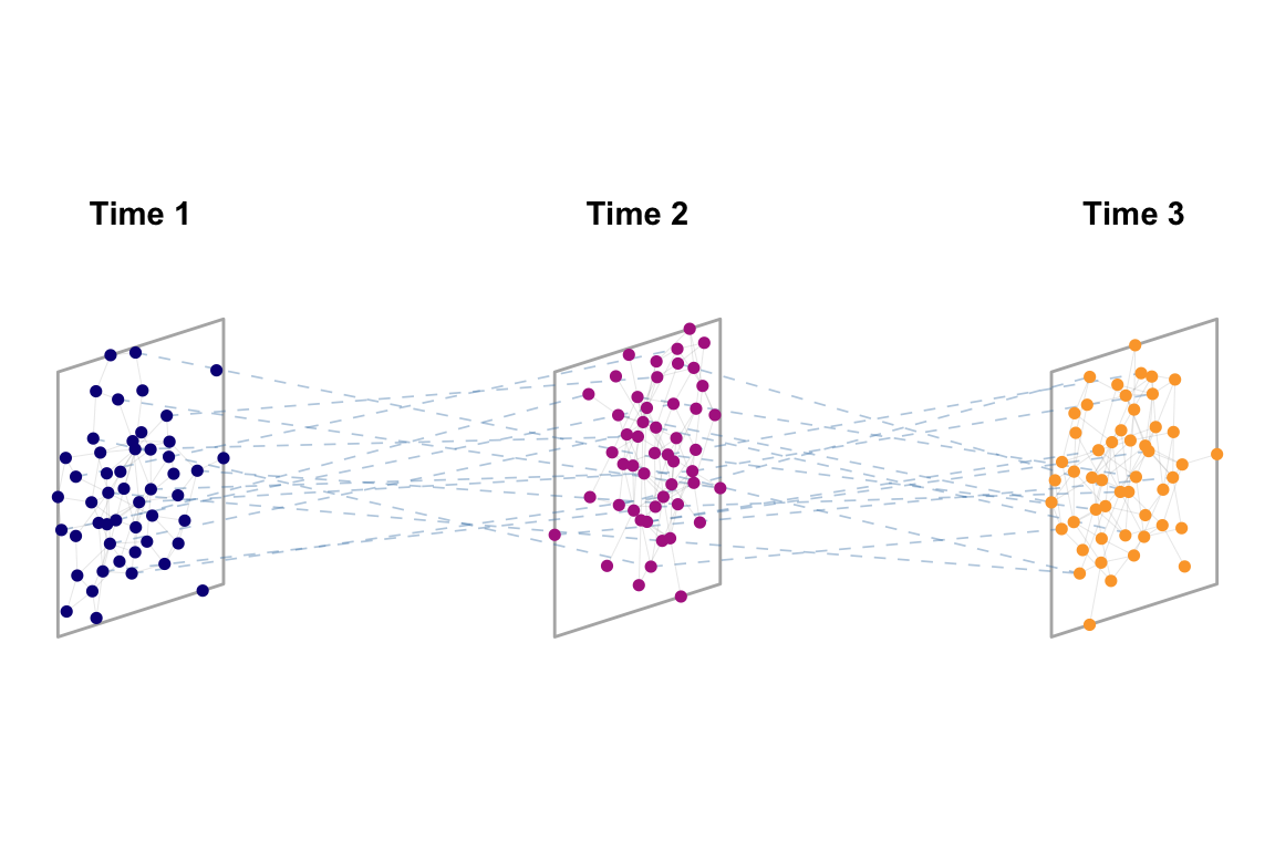

Plot the temporal network you chose to analyse in the last section.

4. Structural properties

MuxViz is largely the most comprehensive packlage fro multilayer network analysis. Here is a list of functions. It is impossible to go through all the structural properties available and you can see the references in the class page for papers and books.

Here is an example with in and out multi-degrees.

mEdges <- as.data.frame(multilayer_kefi$extended_ids[,c(2,1,4,3,5)])
colnames(mEdges)[1:4] <- c("node.from", "layer.from", "node.to", "layer.to")
M <- BuildSupraAdjacencyMatrixFromExtendedEdgelist(mEdges,3,106,T)
out_deg <- GetMultiOutDegree(M, Layers = 3, Nodes = 106, isDirected = T)
in_deg <- GetMultiInDegree(M, Layers = 3, Nodes = 106, isDirected = T)
tibble(out_deg, in_deg) %>% ggplot(aes(in_deg, out_deg))+geom_point()+labs(x='In degree', y='Out degree')+
  geom_abline()+
  xlim(0,85)+
  ylim(0,85)+
  coord_fixed()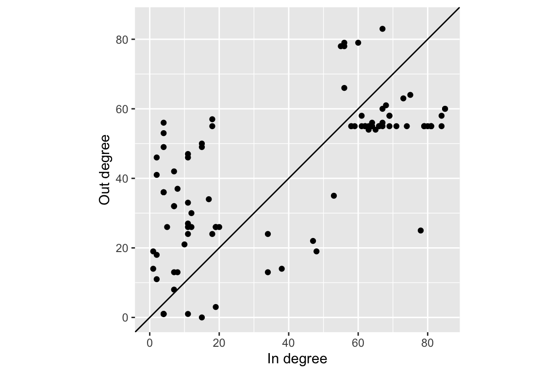

Try to program yourself two metrics from Boccaleti et al 2014:

The total overlap \(O^{\alpha\beta}\) between two layers \(\alpha\) and \(\beta\), defined as the total number of links that are in common between the pair of layers.
The local overlap \(o_i^{\alpha\beta}\) between two layers \(\alpha\) and \(\beta\), defined as the total number of neighbors of node \(i\) that are neighbors in both layers.

5. Aggregating networks

It is sometimes useful to aggregate a multilayer network into a single network. This is actually what has been traditionally done when not enough data were available. There are multiple ways to do so, as in the figure.

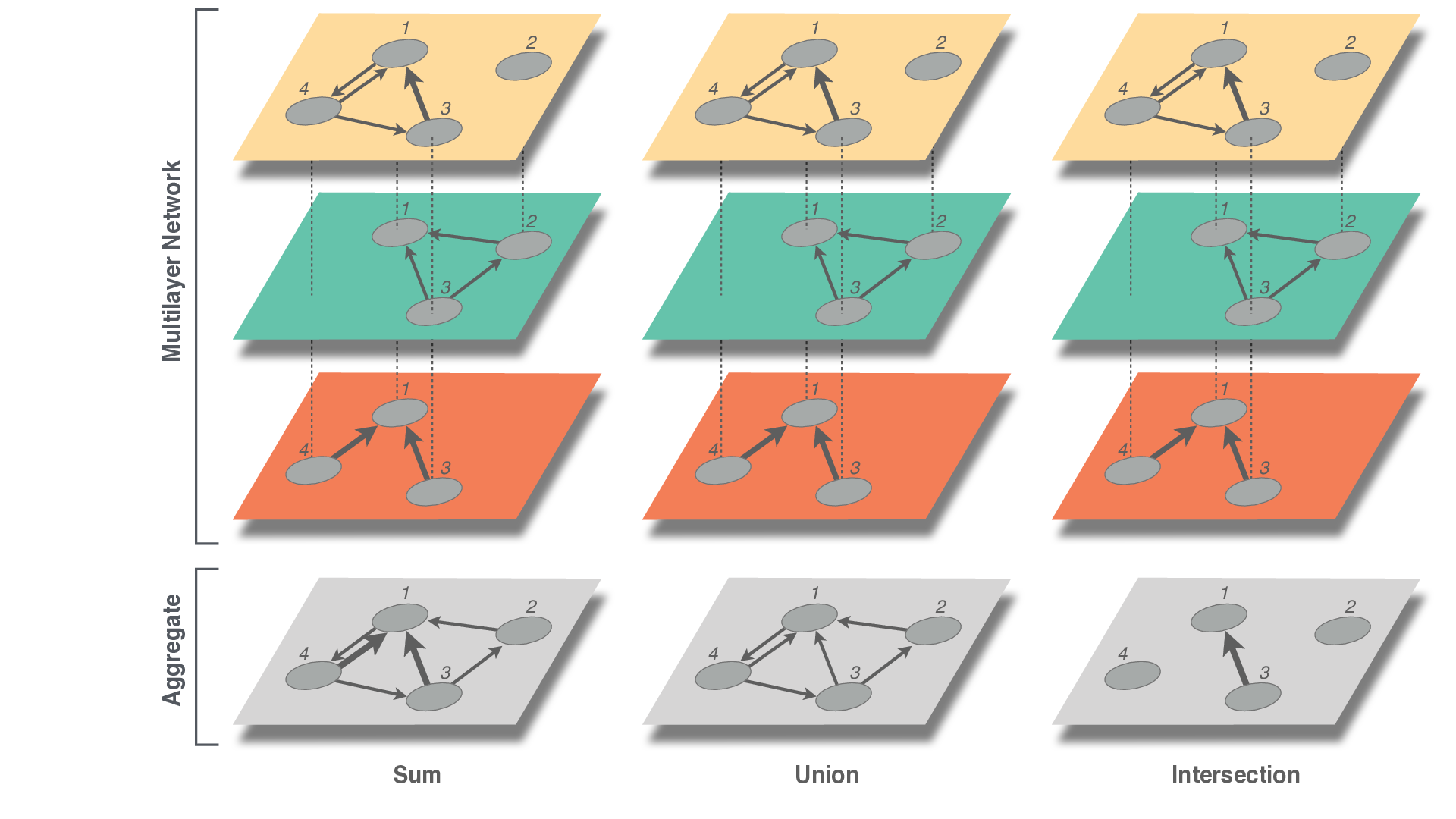
Figure copy-righted to Manlio de Domenico, https://github.com/manlius/muxViz/blob/master/gui-old/theory/README.md

Write code to aggregate in each of these ways.

6. Community detection – Infomap

First, go over the example in the EMLN guide. This example does not have interlayer links so there is a global relax rate set.

Rerun the modularity while varying the global relax rate from 0.05 to 0.95 and record the number of modules. Plot the relationship. Is there a pattern? Can you explain it?

Lab: Multilayer networks

Last update: 03 March, 2026

Code

1. Data structures: Monolayer networks

2. Data structures: Multilayer networks

Multilayer network components

Three representations of a multilayer network

No interlayer links.

Toy example

The multilayer class

Real data

Adding interlayer links

Toy example

Real example with a bipartite network

Converting to supra-adjacency matrices and igraph

Exercise: multilayer data structures

3. Plotting

4. Structural properties

5. Aggregating networks

6. Community detection – Infomap