Lab: Introduction to igraph and data structures
Last update: 03 March, 2026
![]()
Data
We will use some external files during the exercises. Download the data and put it in the exercise folder. You only need to do this once, the file contains data for all the exercises.
Code
A. About this lab
This course requires experience with R and R-studio. Please complete the tutorials if you need to. Some of the material for this lab will be taught in the next class.
B. Packages
There are plenty of R packages dedicated to network analysis in
general and to ecological networks in particular (also for more general
biological networks). In this course we will present several of them,
but you can always choose those that are more convenient to you. We will
especially work with bipartite and igraph.
Let’s make sure you have them installed. Then load them. You can do that
via the Packages tab in R-studio or by typing:
Each of these packages contains many functions for analyzing and
visualizing networks. A great resource for igraph is http://igraph.org/r/doc/. We will cover only a few of
these but once you get the basics you can use any function you want.
Remember to always read the description of the function in the
help file, and if this is a major part of your analysis, go to the
original references. Let’s try one example for getting help.
Note the igraph:: prefix. This tells R that the betweenness
command is from the igraph package, since it also appears
in the sna package, loaded by bipartite.
Note: It is of course impossible to know every command, function, argument and option. Therefore, many times we will rely on our best friend Google to search for solutions and help. Particularly we recommend Stack Exchange (or stack overflow). As an example try searching in google for: “creating binary matrix in r”.
1. igraph basics
Some of this section is based on https://kateto.net/networks-r-igraph.
1.1 Create networks
The code below generates an undirected graph with three edges. The numbers are interpreted as vertex IDs, so the edges are 1—2, 2—3, 3—1.
g1 <- graph(edges=c(1,2, 2,3, 3, 1), n=3, directed=F)
plot(g1) # A simple plot of the network - we'll talk more about plots later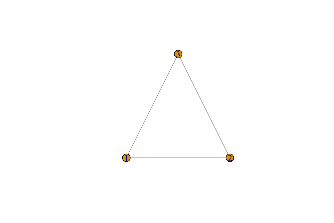
## [1] "igraph"## IGRAPH 6a44e3e U--- 3 3 --
## + edges from 6a44e3e:
## [1] 1--2 2--3 1--3Now directed:
## IGRAPH b0d1b8e D--- 10 3 --
## + edges from b0d1b8e:
## [1] 1->2 2->3 3->1
With named vertices, note the N in the description.
g3 <- graph(c("plankton", "fish1", "plankton", "fish2",
              "fish2", "fish1", "shark", "fish1", "shark", "fish2"), directed=T) # named vertices
plot(g3, edge.arrow.size=.5, vertex.color="gold", vertex.size=15,
     vertex.frame.color="gray", vertex.label.color="black",
     vertex.label.cex=0.8, vertex.label.dist=2, edge.curved=0.2)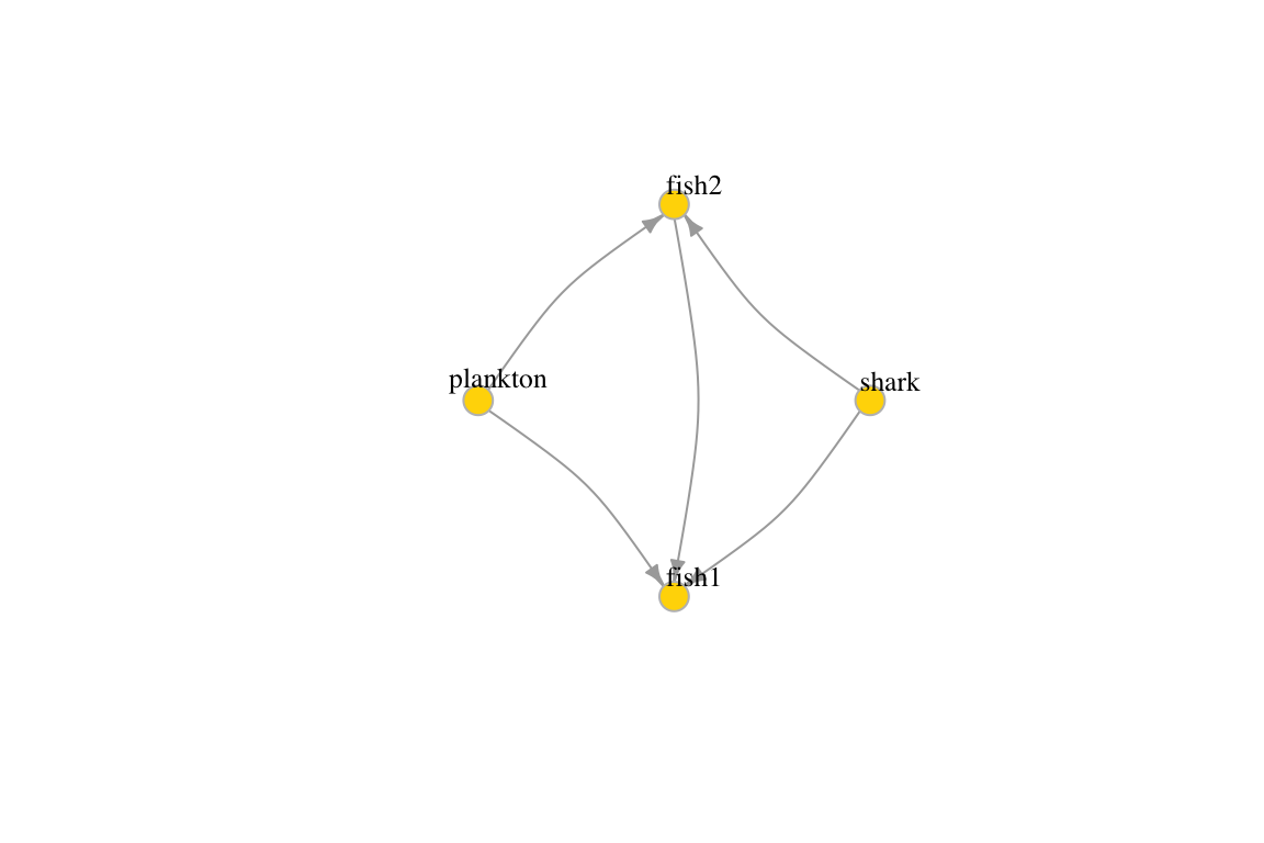
## IGRAPH 24e7c27 DN-- 4 5 --
## + attr: name (v/c)
## + edges from 24e7c27 (vertex names):
## [1] plankton->fish1 plankton->fish2 fish2   ->fish1 shark   ->fish1 shark   ->fish2
1.2 Edge, vertex, and network attributes
The description of an igraph object starts with up to four letters:
- D or U, for a directed or undirected graph
- N for a named graph (where nodes have a name attribute)
- W for a weighted graph (where edges have a weight attribute)
- B for a bipartite (two-mode) graph (where nodes have a type attribute)
The two numbers that follow refer to the number of nodes and edges in the graph. The description also lists node & edge attributes, for example:
- (g/c) - graph-level character attribute
- (v/c) - vertex-level character attribute
- (e/n) - edge-level numeric attribute
Access vertices and edges:
## + 5/5 edges from 24e7c27 (vertex names):
## [1] plankton->fish1 plankton->fish2 fish2 ->fish1 shark ->fish1 shark ->fish2## + 4/4 vertices, named, from 24e7c27:
## [1] plankton fish1 fish2 sharkAdd attributes to the network, vertices, or edges:
## [1] "plankton" "fish1" "fish2" "shark"V(g3)$taxonomy <- c("diatoms", "Genus sp1", "Genus sp2", "Genus sp3")
E(g3)$type <- "predation" # Edge attribute, assign "email" to all edges
E(g3)$weight <- c(1,1.5,4,10, 6)
edge_attr(g3)## $type
## [1] "predation" "predation" "predation" "predation" "predation"
##
## $weight
## [1] 1.0 1.5 4.0 10.0 6.0## $name
## [1] "plankton" "fish1" "fish2" "shark"
##
## $taxonomy
## [1] "diatoms" "Genus sp1" "Genus sp2" "Genus sp3"## $name
## [1] "My 1st food web"## IGRAPH 24e7c27 DNW- 4 5 -- My 1st food web
## + attr: name (g/c), name (v/c), taxonomy (v/c), type (e/c), weight (e/n)
## + edges from 24e7c27 (vertex names):
## [1] plankton->fish1 plankton->fish2 fish2 ->fish1 shark ->fish1 shark ->fish21.3 Bipartite graphs
Bipartite networks have an additional type attribute
with FALSE for the nodes of the first set and TRUE for nodes of the
second set.
## IGRAPH 7db5e8b U--B 10 5 --
## + attr: type (v/l)
## + edges from 7db5e8b:
## [1] 1-- 2 3-- 4 5-- 6 7-- 8 9--10## $type
## [1] FALSE TRUE FALSE TRUE FALSE TRUE FALSE TRUE FALSE TRUE## [1] TRUE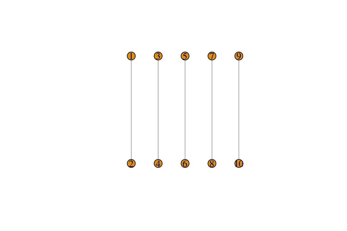
2. Data structures for unipartite networks
Networks can be represented using several data structures. Knowing
these data structures and how to transform from one to another is a very
handy skill as even within R different packages use
different structures. The two main data structures are matrices
and edge lists and we will focus on those. These are general
and not specific to R. There are, however, some data structures which
are specific to different R packages and we will deal with those as we
go along.
Note: During this section we will meet some basics of
igraph. While it is not the main goal of this section, it
is a good intro.
2.1 Networks as matrices
Unweighted networks
Let’s see an example for an undirected graph:
A_u <- matrix(c(0,1,1,0,0, # An example input matrix
              1,0,0,1,1,
              1,0,0,0,0,
              0,1,0,0,0,
              0,1,0,0,0),5,5, byrow=F)
isSymmetric(A_u)
## [1] TRUE
And for a directed graph:
A_d <- matrix(c(0,1,1,0,1, # An example input matrix
              1,0,0,1,1,
              1,0,0,0,0,
              0,1,0,0,0,
              0,1,1,0,0),5,5, byrow=F)
isSymmetric(A_d)
## [1] FALSE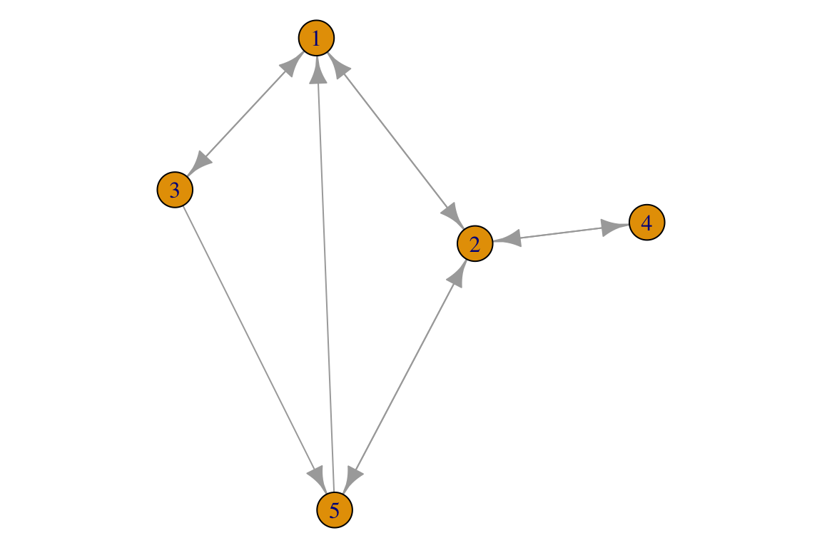
1. Try to add a self-loop to one of the networks.
2. Try to create a directed graph in which there is a singleton (a node without any interactions).
Weighted networks
For the sake of the example, we will create a network with some random edge weights. Again we will have 5 nodes with 4 edges in an undirected network.
A_w <- matrix(c(0,1,1,0,0, # An example input matrix
              1,0,0,1,1,
              1,0,0,0,0,
              0,1,0,0,0,
              0,1,0,0,0),5,5, byrow=F)
random_weights <- round(rnorm(10, 10, 4),2) # take weights from a normal distribution.
A_w[lower.tri(A_w)] <- A_w[lower.tri(A_w)]*random_weights # Fill the lower traiangle
A_w <- A_w+t(A_w) # This makes the matrix symmetric
isSymmetric(A_w)
## [1] TRUE## [1] 14.67 12.16 10.98 6.60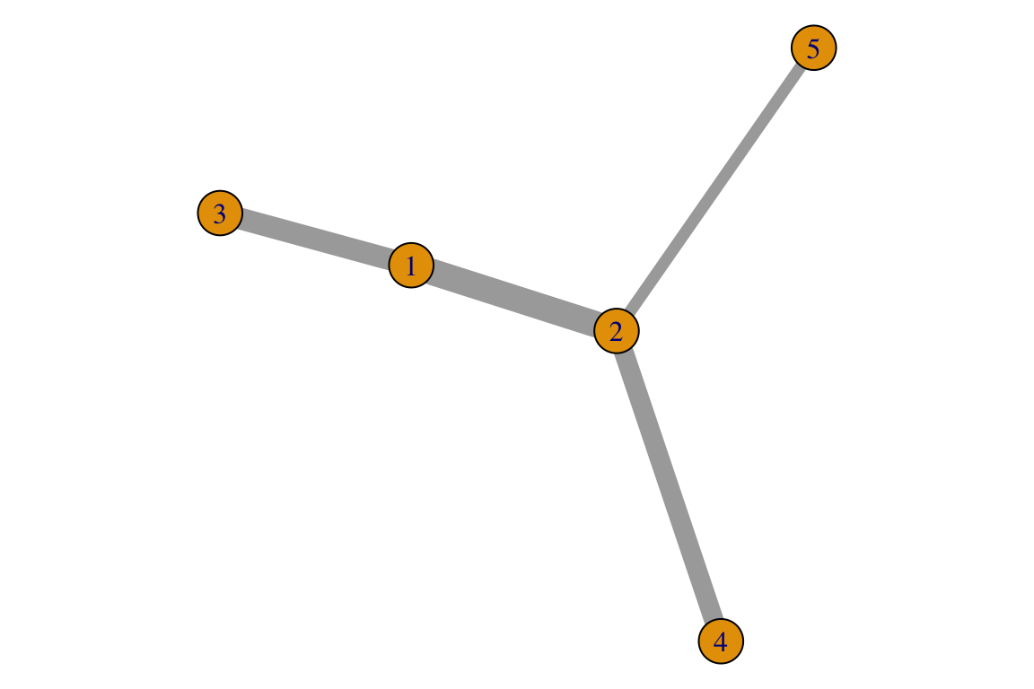
3. Try do follow the code above to create a directed weighted network.
Note that in this course we will refer to an edge or a link as a component of the network and to an interaction as an ecological interaction. For example, predation is an ecological interaction represented as an edge in a food web.
4. What can edge weights be in ecological networks? Try to think of at least 3 diffeterent measures for an ecological interaction. If you work with other network types, answer the question according to your domain of expertise.
2.2 Networks as edge lists
Unweighted
Edge lists for unweighted networks are basically a table with 2 columns and as many rows as there are interactions. A simple example would be the equivalent for the network we previously represented with a matrix:
L_u <- data.frame(i=c(1,1,2,2),
                j=c(2,3,4,5))
g <- igraph::graph.data.frame(L_u, directed = F)
par(mar=c(0,0,0,0))
plot(g)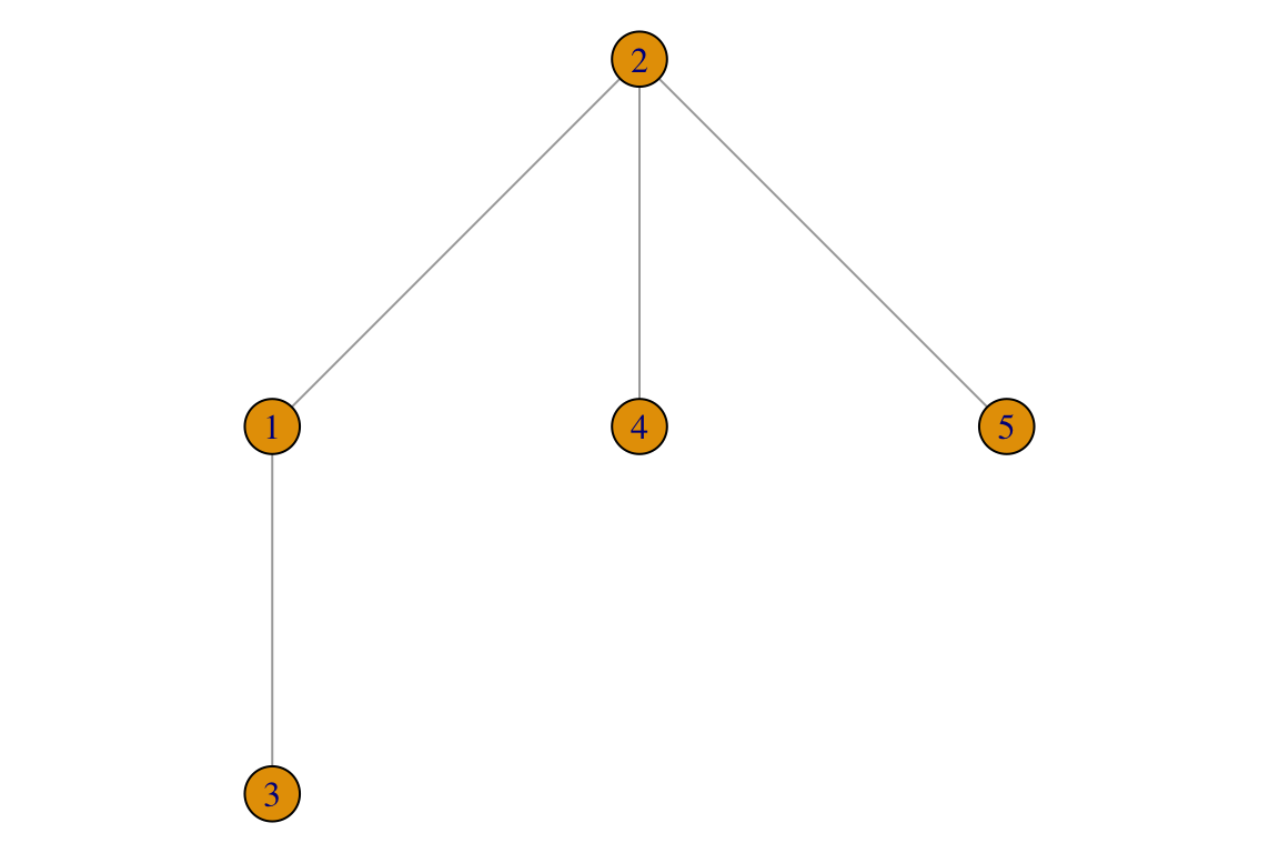
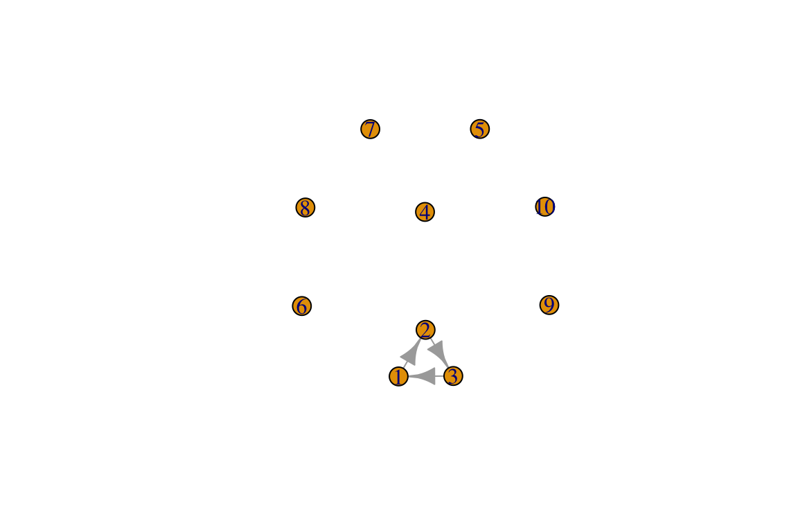
For the directed network:
L_u <- data.frame(i=c(1, 1, 2, 2, 2, 3, 3, 4, 5, 5),
                j=c(2, 3, 1, 4, 5, 1, 5, 2, 1, 2))
g <- igraph::graph.data.frame(L_u, directed = T)
par(mar=c(0,0,0,0))
plot(g)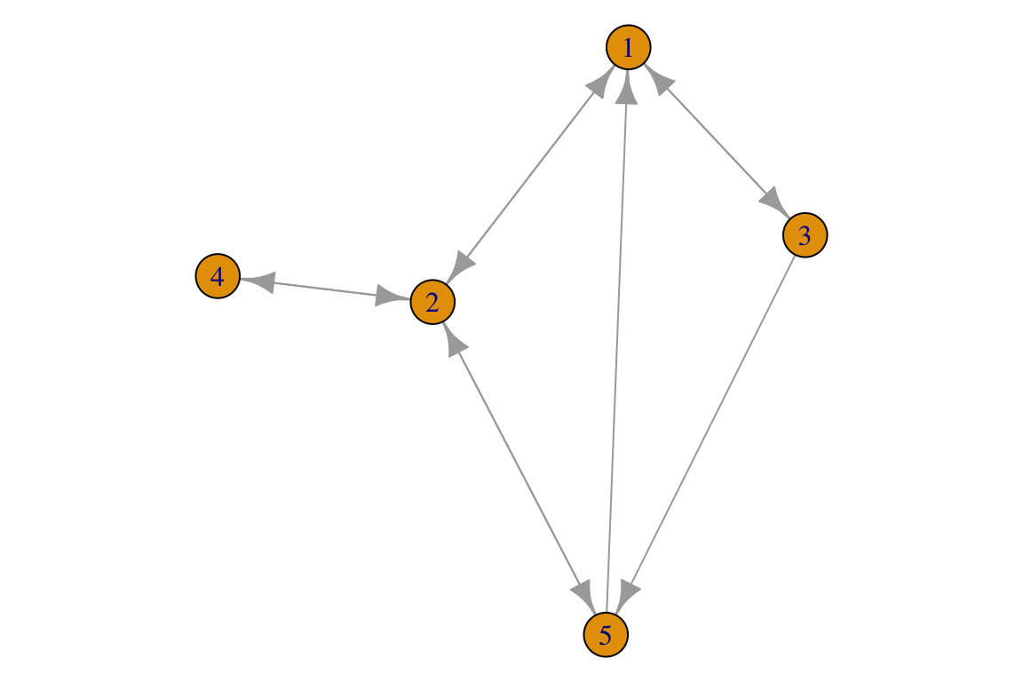
Note that for directed networks it may be more convenient to label
the columns using from and to than
i and j.
5. Try to add a self-loop to the edge list, using from and to as column names.
Weighted
An edge list for a weighted network requires an additional column for edge weights. Following the previous examples for undirected networks:
L_w <- data.frame(i=c(1,1,2,2),
                j=c(2,3,4,5),
                weight=round(rnorm(4, 10, 4),2) # take weights from a normal distribution.
                )
g <- igraph::graph.data.frame(L_w, directed = F)
E(g)$weight
## [1] 4.70 6.17 20.32 3.95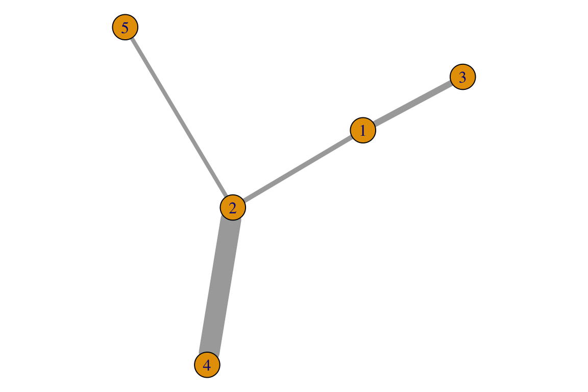
And for directed networks:
L_wd <- data.frame(from=c(1, 1, 2, 2, 2, 3, 3, 4, 5, 5),
                to=c(2, 3, 1, 4, 5, 1, 5, 2, 1, 2),
                weight=round(rnorm(10, 1, 0.2),2))
g <- igraph::graph.data.frame(L_wd, directed = T)
g
## IGRAPH 146eb9c DNW- 5 10 --
## + attr: name (v/c), weight (e/n)
## + edges from 146eb9c (vertex names):
## [1] 1->2 1->3 2->1 2->4 2->5 3->1 3->5 4->2 5->1 5->2## [1] 0.87 1.12 0.97 0.64 1.06 0.79 1.01 0.55 0.84 0.72par(mar=c(0,0,0,0))
plot(g, edge.width=log(E(g)$weight)*10, # possible to rescale edge weights when plotting
edge.arrow.size=1.2,
edge.curved=0.5,
edge.color='black')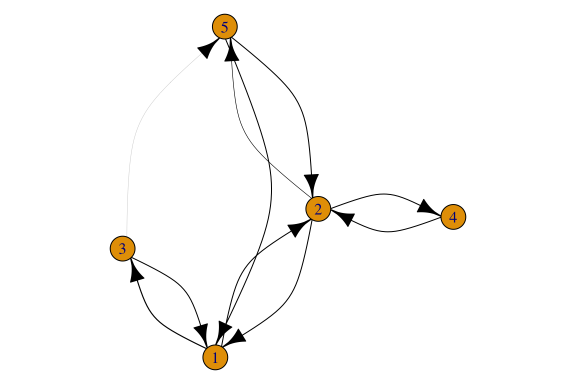
6. What are the advantages/disadvantages of edge lists compared to matrices?
2.3 Converting between matrices and edge lists
Because different implementations use different data structures, converting between these two is rather important. We will first do that in igraph. Working with igraph is fast (especially when working with large and/or dense networks), economic in code, flexible and in most cases delivers what we want. So it is highly recommended. But that is cheating!!! So we will also program this ourselves.
First, note that you can see both structures from the igraph object:
## 5 x 5 sparse Matrix of class "dgCMatrix"
##     Sp1 Sp2 Sp3 Sp4 Sp5
## Sp1   .   5   2   .   .
## Sp2   7   .   .   0   6
## Sp3   4   .   .   .   3
## Sp4   .   6   .   .   .
## Sp5 3 1 . . .## Sp1 Sp2 Sp3 Sp4 Sp5
## Sp1 0 5 2 0 0
## Sp2 7 0 0 0 6
## Sp3 4 0 0 0 3
## Sp4 0 6 0 0 0
## Sp5 3 1 0 0 0## from to weight
## 1 Sp1 Sp2 5
## 2 Sp1 Sp3 2
## 3 Sp2 Sp1 7
## 4 Sp2 Sp4 0
## 5 Sp2 Sp5 6
## 6 Sp3 Sp1 4
## 7 Sp3 Sp5 3
## 8 Sp4 Sp2 6
## 9 Sp5 Sp1 3
## 10 Sp5 Sp2 1## name
## Sp1 Sp1
## Sp2 Sp2
## Sp3 Sp3
## Sp4 Sp4
## Sp5 Sp5Matrix to edge list:
##       [,1]  [,2]  [,3]  [,4] [,5]
## [1,]  0.00 14.67 12.16  0.00  0.0
## [2,] 14.67  0.00  0.00 10.98  6.6
## [3,] 12.16  0.00  0.00  0.00  0.0
## [4,]  0.00 10.98  0.00  0.00  0.0
## [5,]  0.00  6.60  0.00  0.00  0.0
g <- igraph::graph.adjacency(A_w, mode = 'directed', weighted = T)
L <- igraph::as_data_frame(g, what = 'edges')
L## from to weight
## 1 1 2 14.67
## 2 1 3 12.16
## 3 2 1 14.67
## 4 2 4 10.98
## 5 2 5 6.60
## 6 3 1 12.16
## 7 4 2 10.98
## 8 5 2 6.60Edge list to matrix:
##    from to weight
## 1     1  2   0.87
## 2     1  3   1.12
## 3     2  1   0.97
## 4     2  4   0.64
## 5     2  5   1.06
## 6     3  1   0.79
## 7     3  5   1.01
## 8     4  2   0.55
## 9     5  1   0.84
## 10    5  2   0.72
g <- igraph::graph.data.frame(L_wd, directed = T)
A <- igraph::as_adjacency_matrix(g, attr = 'weight', sparse=F)
A## 1 2 3 4 5
## 1 0.00 0.87 1.12 0.00 0.00
## 2 0.97 0.00 0.00 0.64 1.06
## 3 0.79 0.00 0.00 0.00 1.01
## 4 0.00 0.55 0.00 0.00 0.00
## 5 0.84 0.72 0.00 0.00 0.007. Try programming a function that takes a matrix and returns an edge list. Note that it may be important if the matrix is directed or weighted.
8. Try programming a function that takes an edge list and returns a matrix. Note that it may be important if the matrix is directed or weighted.
Working with empirical data
It is not trivial to work with external data, especially when it is
spread across several files. Usually you will need an ad-hoc way to deal
with your data, so as you go you will definitely master your data
management skills in R :)
3. Unipartite networks
Food webs are a classic example of a unipartite network and are by far the most studied kind of netwok in ecology. As an example, let’s explore the Otago Lake (NZ) food web. The description of the data is a data paper in Ecological Archives E092-173-D1.
9. Browse through the metadata. Name 5 variables that are used as attributes. What kinds of attributes. can nodes in networks that you would work with have?
We have already downloaded the nodes and links for this class. Let’s load the network:
otago_nodes <- read.csv('data/Otago_Data_Nodes.csv')
otago_links <- read.csv('data/Otago_Data_Links.csv')
otago_nodes[1:4,1:6]
## NodeID SpeciesID StageID Stage Species.StageID WorkingName
## 1 1 1 1 Adult 1.1 Phytoplankton
## 2 2 2 1 Adult 2.1 Epipellic Flora
## 3 3 3 1 Adult 3.1 Macroalgae/Seagrass
## 4 4 4 1 Adult 4.1 Zooplankton## ConsumerNodeID ResourceNodeID ConsumerSpeciesID ResourceSpeciesID ConsumerSpecies.StageID ResourceSpecies.StageID
## 1 4 1 4 1 1 1
## 2 4 4 4 4 1 1
## 3 4 6 4 6 1 1
## 4 5 1 5 1 1 1
## LinkTypeID LinkType
## 1 1 Predation
## 2 1 Predation
## 3 1 Predation
## 4 1 PredationAs you can see these are data frames, which contain a lot of
information besides a simple network. igraph can handle
many ways to import data to generate igraph network objects. Let’s
import that data frame (we have seen that previously in the lab):
# Import to igraph, including edge and node attributes
otago_web <- graph.data.frame(otago_links, vertices = otago_nodes, directed = T)
The graph. commands import different kinds of data
structures. The advantage of importing a data frame is that igraph also
imports the attributes of the edges. The edge attributes are
imported from the edge data frame (otago_links) and the
node attributes are imported using the vertices= argument
pointing to a data frame with node attributes. We can access edge and
vertex attributes with E and V,
respectively.
##  [1] "ConsumerSpeciesID"       "ResourceSpeciesID"       "ConsumerSpecies.StageID" "ResourceSpecies.StageID"
##  [5] "LinkTypeID"              "LinkType"                "LinkEvidence"            "LinkEvidenceNotes"
##  [9] "LinkFrequency"           "LinkN"                   "DietFraction"            "ConsumptionRate"
## [13] "VectorFrom" "PreyFrom"## [1] "Predation" "Parasitic Castration" "Macroparasitism"
## [4] "Commensalism" "Trophically Transmitted Parasitism" "Concomitant Predation on Symbionts"## [1] "name" "SpeciesID" "StageID" "Stage"
## [5] "Species.StageID" "WorkingName" "OrganismalGroup" "NodeType"
## [9] "Resolution" "ResolutionNotes" "Feeding" "Lifestyle.stage."
## [13] "Lifestyle.species." "ConsumerStrategy.stage." "System" "HabitatAffiliation"
## [17] "Mobility" "Residency" "NativeStatus" "BodySize.g."
## [21] "BodySizeEstimation" "BodySizeNotes" "BodySizeN" "Biomass.kg.ha."
## [25] "BiomassEstimation" "BiomassNotes" "Kingdom" "Phylum"
## [29] "Subphylum" "Superclass" "Class" "Subclass"
## [33] "Order" "Suborder" "Infraorder" "Superfamily"
## [37] "Family" "Genus" "SpecificEpithet" "Subspecies"
## [41] "NodeNotes"## [1] "Phytoplankton" "Epipellic Flora" "Macroalgae/Seagrass" "Zooplankton" "Meiofauna"
## [6] "Bacteria"The values of V(otago_web)$name are those from the
ConsumerNodeID and ResourceNodeID columns in
otago_links.
10. Try to load a new food web, the Bahia Falsa. The Bahia Falsa data set is described in http://datadryad.org/resource/doi:10.5061/dryad.b8r5c
3.1 Plotting with igraph
Let’s try to plot. We have already seen how to call a basic plot:
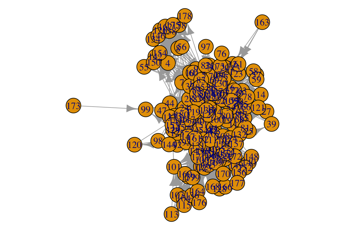
What a mess… We can definitely make this nicer!!! There are many many ways to tweak igraph plots. Check out http://igraph.org/r/doc/plot.common.html or https://kateto.net/networks-r-igraph. Of course our best friend Stack Overflow will have many answers for specific questions.
Here is a nicer plot with some tweaks:
par(mar=c(0,0,0,0))
plot(otago_web, vertex.size=3, edge.arrow.size=0.4, vertex.label=NA, layout=layout.circle)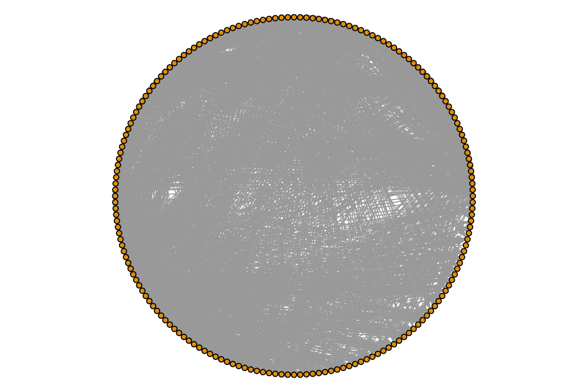
Now, let’s try to both set link attributes and use them for plotting. We will color edges by the type of interactin they represent:
E(otago_web)$color <- "grey" # First, we set a default color
E(otago_web)[otago_links$LinkType == 'Predation']$color <- "black"
E(otago_web)[otago_links$LinkType == 'Macroparasitism']$color <- "blue"
E(otago_web)[otago_links$LinkType == 'Trophic Transmission']$color <- "red"
# Now plot
par(mar=c(0,0,0,0))
plot(otago_web, vertex.size=2, edge.arrow.size=0.2, vertex.label=NA, layout=layout.circle)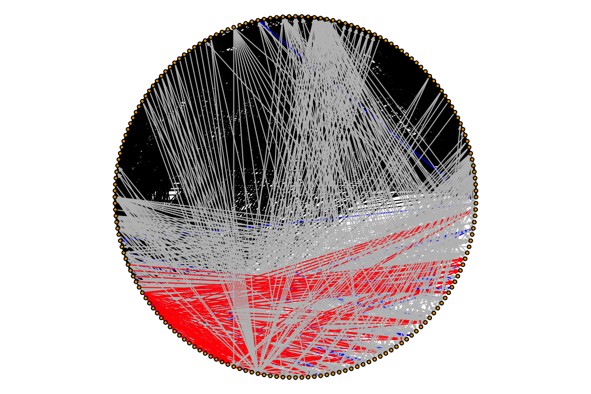
In food webs, species can be divided into three main trophic groups: basal, intermediate and top predators. Let’s try to clasify the species on the Otago food web.
# Basal species (those that do not consume) -- do not have incoming links
basal <- which(igraph::degree(otago_web, mode = 'in') == 0)
# Top species do not have outgoing links
top <- which(igraph::degree(otago_web, mode = 'out') == 0)
# Intermediate are all the rest
interm <- V(otago_web)[which(!V(otago_web) %in% c(basal,top))]
# Are all the nodes included?
all(c(basal,top,interm) %in% V(otago_web))
## [1] TRUE## [1] TRUENow let’s try to re-plot the food web using these classifications. We will use our own layout, which is a matrix with coordinates.
V(otago_web)$troph_pos <- rep(0,length(V(otago_web)))
V(otago_web)$troph_pos[which(V(otago_web)$name %in% basal)] <- 1
V(otago_web)$troph_pos[which(V(otago_web)$name %in% top)] <- 3
V(otago_web)$troph_pos[which(V(otago_web)$name %in% interm)] <- 2
# create a matrix forthe layout coordinates.
coords <- matrix(nrow=length(V(otago_web)), ncol=2) #
# The x positions are randomly selected
coords[,1] <- runif(length(V(otago_web)))
# The y positions are the trophoc positions
coords[,2] <- V(otago_web)$troph_pos
par(mar=c(0,0,0,0))
plot(otago_web,layout=coords,
            vertex.color=V(otago_web)$troph_pos,
            vertex.label=NA,
            vertex.size=8,
            edge.color='black',
            edge.arrow.size=.3,
            edge.width=.5)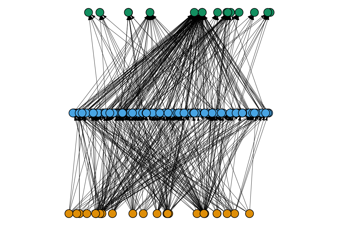
11. Try to set other node and edge attributes
based on otago_nodes and otago_links. For
example, try to color nodes by OrganismalGroup and plot.
Does the organismal group correspond to the trophic position?
4. Bipartite networks
4.1 Using data from the bipartite package
The package bipartite has several data sets implemented.
Let’s try one:
## [1] "matrix" "array"## Coleoptera.spec1 Coleoptera.spec2 Coleoptera.spec3 Coleoptera.spec4
## Agrimonium.eupatorium 0 0 0 0
## Leontodon.autumnalis 0 0 0 0
## Lotus.corniculatus 0 0 0 0
## Medicago.lupulina 0 0 0 0Obviously, it is extremely important we understand the data we are
looking at and working with. What are the species? what are the edges?
Where were the data collected? How? For the built-in data sets we can
just use the help (e.g., ?memmott1999. For other data sets
it is necessary to go to the original publication. A bipartite network
has two guilds. As a convention, the rows are the “lower” trophic level
(e.g., plants, hosts) and the columns are the “higher” trophic level
(e.g., pollinators, parasites).
plant_species <- rownames(memmott1999)
flower_visitor_species <- colnames(memmott1999)
head(plant_species, 3)
## [1] "Agrimonium.eupatorium" "Leontodon.autumnalis" "Lotus.corniculatus"## [1] "Coleoptera.spec1" "Coleoptera.spec2" "Coleoptera.spec3"12. Try to load a different data set. Where can you find available ones?.
4.2 Visualizaing bipartite data
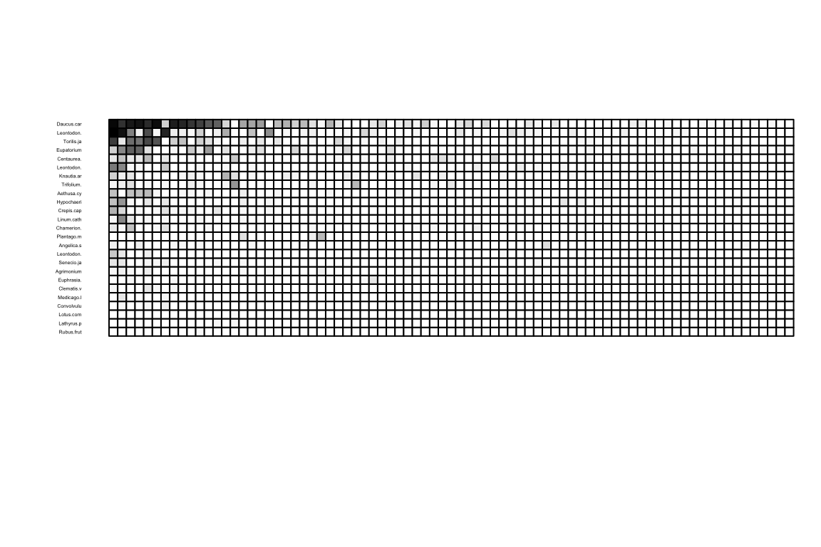
We can visualize the incidence matrix using:
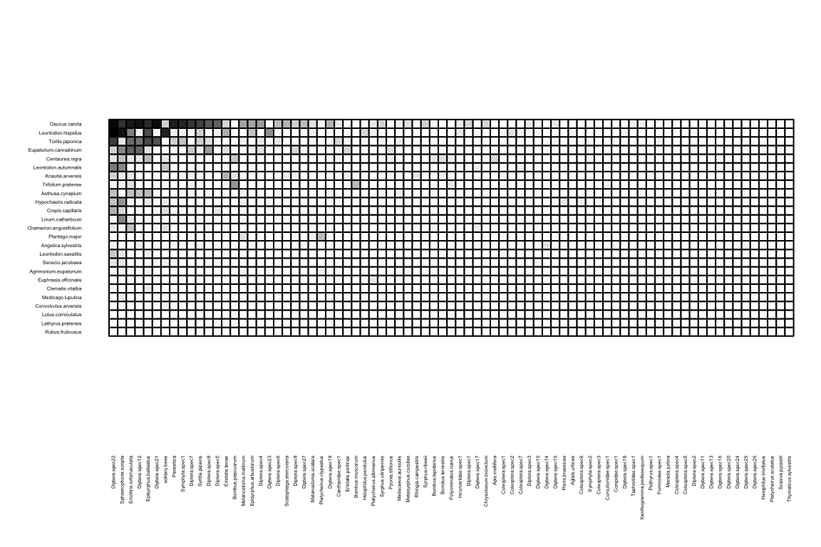
Can you see the different hues? This is a quantitative network, where matrix cell values indicate the strength of an ecological interaction. Sometimes it is useful to look only at the edges (regardless of values), in a binary network. So we only want to see those entries larger than 0.
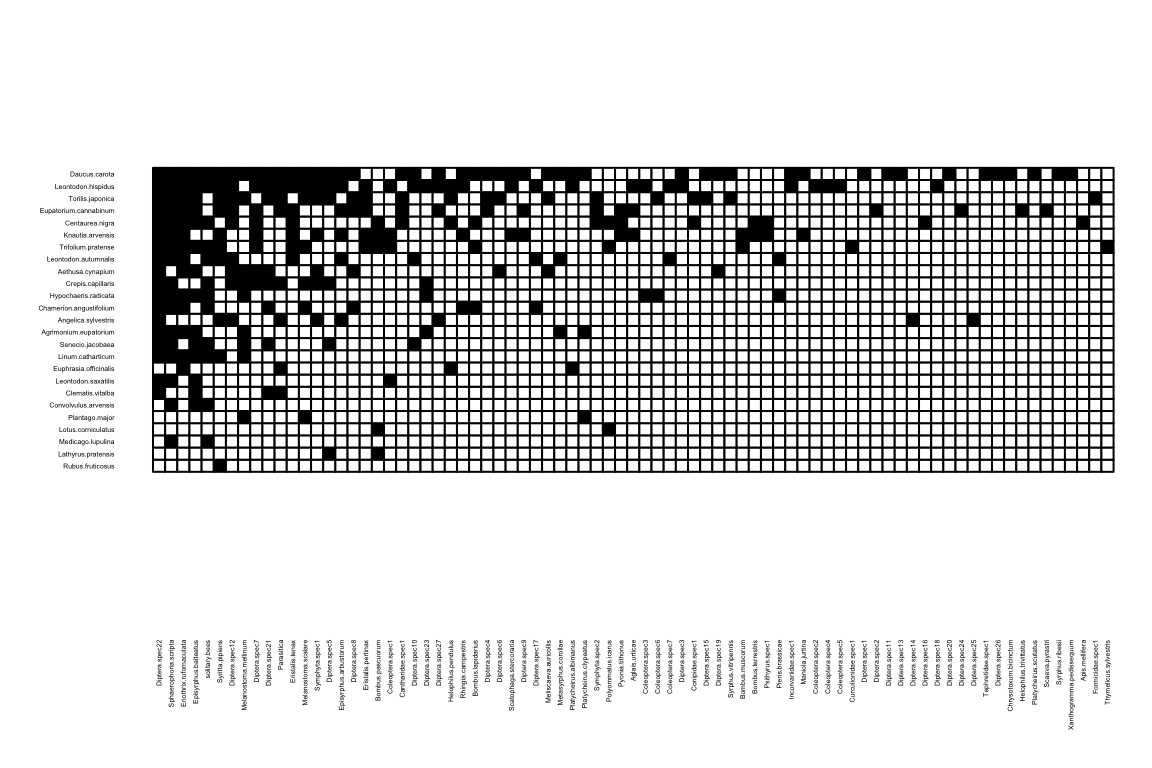
visweb works OK for small networks, although as you can see, it may
need some tweaking to improve the plotting… We can do that by using the
function’s options, just like with any other function in R.
An examplpe:
Another way to plot a bipartite network is by connecting nodes with lines:
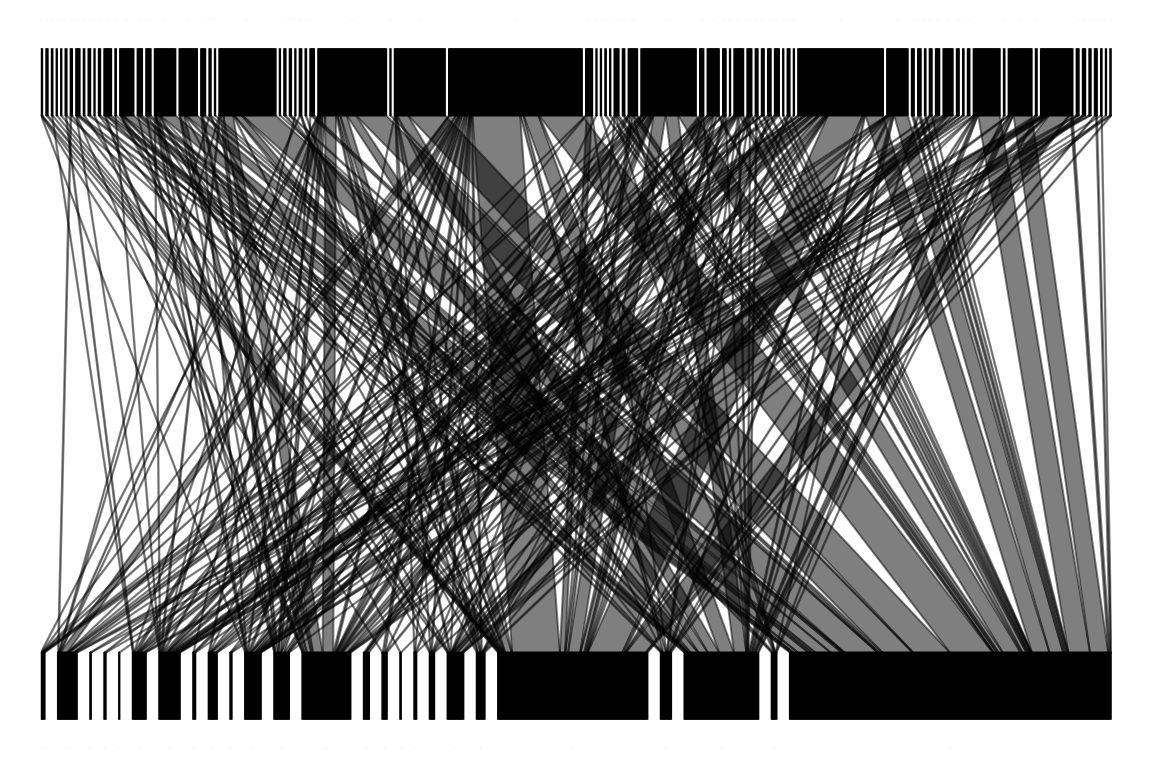
13. Can you say something about the network using this representation? What does it reveal just by looking?
14. Try to browse through the options in plotweb and tweak the plot.
4.3 Importing data
Let’s start with a simple example. This is a host-parasite network from http://datadryad.org/resource/doi:10.5061/dryad.jf3tj/4.
This file is not as clean. Let’s take a look and prepare it.
##                         X Num..of.hosts.sampled Ctenophthalmus.wagneri Nosopsyllus.consimilis
## 1 Clethrionomys glareolus                  5209                   1748                    337
## 2      Apodemus uralensis                 15198                   1408                    893
## 3        Microtus arvalis                  1920                    494                    193
## 4           Sorex araneus                   856                    237                      6
The first column is species names and the second is the number of hosts sampled, and the rest of the columns are the parasites. Columns 1 and 2 are not part of the network itself. So we will put the hosts as the row names and remove the number of hosts sampled. We also want the data as a matrix, rather than a data frame.
rownames(ural_data) <- ural_data[,1] # Set row names
num_hosts_sampled <- ural_data[,2] # save in a variable
ural_data <- ural_data[,-2] # remove column
ural_data <- ural_data[,-1] # remove column
class(ural_data) # This is a data frame!
## [1] "data.frame"## Ctenophthalmus.wagneri Nosopsyllus.consimilis Megabothris.turbidus Amphipsylla.rossica
## Clethrionomys glareolus 1748 337 811 144
## Apodemus uralensis 1408 893 414 41
## Microtus arvalis 494 193 97 177
## Sorex araneus 237 6 20 415. Try to plot the Ural Valley data.
4.4 Converting between data structures for bipartite networks
Bipartite networks have two sets of nodes, and this must be taken into account when representing the data in edge lists or incidence matrices.
Crucial exercise 1: Try to represent the
memmott1999 data as a matrix, edge list and write
algorithms that convert between these two.
Crucial exercise 2: Import the
memmott1999 data as an igraph object. Then explore the
attributes.
5. Visualizations with ggnetwork
While we use igraph for plotting, there may be a more convenient way.
Check out the ggnetwork package: https://cran.r-project.org/web/packages/ggnetwork/vignettes/ggnetwork.html.
6. External resources for data
17. Try to obtain 2 data sets (one unipartite and one bipartite), load them and plot them.