Lab: Basic structural metrics
Last update: 03 March, 2026
![]()
1. Introduction
There is an endless number of metrics for network structure in the general network science, and several more developed particularly for ecological networks. We will naturally focus on the most relevant and popular ones. It is very useful however to have a reference for the most popular ones. In the context of ecology, two papers are particularly useful:
- Dormann CF, Fründ J, Blüthgen N, Gruber B. Indices, graphs and null models: analyzing bipartite ecological networks. The Open Ecology Journal. 2009;2: 7–24.
- Delmas E, Besson M, Brice M-H, Burkle LA, Dalla Riva GV, Fortin M-J, et al. Analysing ecological networks of species interactions: Analyzing ecological networks. Biol Rev. 2019;94: 16–36.
2. Bipartite networks
2.1 Some basic network metrics
Dormann et al. (2009, The Open Ecology Journal) classified bipartite network metrics into: 1. Metrics based on unweighted links 2. Metrics based on weighted links
Here are a few examples (see comments in code to learn what these are).
Calculate metrics:
data(olesen2002flores) # Check out the help for information on this data set!
olesen2002flores_binary <- 1 * (olesen2002flores > 0) # Make the data binary (unweighted)
I <- nrow(olesen2002flores_binary) # Number of lower level species (e.g., hosts, plants)
J <- ncol(olesen2002flores_binary) # Number of higher level species (e.g., parasites, pollinators)
S <- I + J # Total number of species, aka: Network size
L <- sum(olesen2002flores_binary > 0) # Number of edges in the network
A_i <- rowSums(olesen2002flores_binary) # The degree of hosts
A_j <- colSums(olesen2002flores_binary) # The degree of parasites
C <- L / (I * J) # Connectance
# Clustering coefficient higher level (the number of realized links
# divided by the number of possible links for each species)
cc_high <- colSums(olesen2002flores_binary) / nrow(olesen2002flores_binary)
# Clustering coefficient lower level
# (the number of realized links divided by the number of possible links for each species)
cc_low <- rowSums(olesen2002flores_binary) / ncol(olesen2002flores_binary)
In a weighted network we can use strength instead of degree:
S_i <- rowSums(olesen2002flores) # Node strength of hosts
S_j <- colSums(olesen2002flores) # Node strength of parasites
1. Try to calculate these metrics for the
memmott1999 data.
2. Plot the degree and strength distributions
3. Calculate other metrics. Where did you find them?
2.2 Built-in metrics in bipartite
We can of course, write code to calculate each metric but
bipartite has many already implemented. The functions
specieslevel, grouplevel and
networklevel calculate metrics at these respective network
levels. For example:
##  [1] "degree"                        "normalised.degree"             "species.strength"
##  [4] "interaction.push.pull"         "nestedrank"                    "PDI"
##  [7] "resource.range"                "species.specificity.index"     "PSI"
## [10] "node.specialisation.index.NSI" "betweenness"                   "weighted.betweenness"
## [13] "closeness"                     "weighted.closeness"            "Fisher.alpha"
## [16] "partner.diversity"             "effective.partners"            "proportional.generality"
## [19] "proportional.similarity" "d"## [1] 6 4 1 3 3 4 3 2 1 1 1 1## number.of.species.HL number.of.species.LL mean.number.of.links.HL
## 12.0000000 10.0000000 3.8586479
## mean.number.of.links.LL mean.number.of.shared.partners.HL mean.number.of.shared.partners.LL
## 4.4582968 0.7121212 0.8222222
## cluster.coefficient.HL cluster.coefficient.LL weighted.cluster.coefficient.HL
## 0.3858648 0.3715247 0.2701252
## weighted.cluster.coefficient.LL niche.overlap.HL niche.overlap.LL
## 0.2148559 0.2288755 0.2205265
## togetherness.HL togetherness.LL C.score.HL
## 0.1496212 0.1534722 0.5311448
## C.score.LL V.ratio.HL V.ratio.LL
## 0.5455247 1.4745763 1.7346939
## discrepancy.HL discrepancy.LL extinction.slope.HL
## 14.0000000 14.0000000 2.7303650
## extinction.slope.LL robustness.HL robustness.LL
## 2.1356865 0.6449911 0.5729366
## functional.complementarity.HL functional.complementarity.LL partner.diversity.HL
## 900.4271365 854.6445694 0.9325640
## partner.diversity.LL generality.HL vulnerability.LL
## 1.1013382 2.7505169 3.4163571## connectance web asymmetry links per species
## 0.25000000 0.09090909 1.36363636
## number of compartments compartment diversity cluster coefficient
## 1.00000000 NA 0.25000000
## modularity Q nestedness NODF
## 0.49693484 26.73800218 35.96096096
## weighted nestedness weighted NODF spectral radius
## 0.41696529 23.27327327 200.24180974
## interaction strength asymmetry specialisation asymmetry linkage density
## 0.06921118 -0.03946187 3.08343699
## weighted connectance Fisher alpha Shannon diversity
## 0.14015623 5.64810846 2.99270826
## interaction evenness Alatalo interaction evenness H2
## 0.62510985 0.76748398 0.53335441
## number.of.species.HL number.of.species.LL mean.number.of.shared.partners.HL
## 12.00000000 10.00000000 0.71212121
## mean.number.of.shared.partners.LL cluster.coefficient.HL cluster.coefficient.LL
## 0.82222222 0.38586479 0.37152473
## weighted.cluster.coefficient.HL weighted.cluster.coefficient.LL niche.overlap.HL
## 0.27012517 0.21485594 0.22887547
## niche.overlap.LL togetherness.HL togetherness.LL
## 0.22052649 0.14962121 0.15347222
## C.score.HL C.score.LL V.ratio.HL
## 0.53114478 0.54552469 1.47457627
## V.ratio.LL discrepancy.HL discrepancy.LL
## 1.73469388 14.00000000 14.00000000
## extinction.slope.HL extinction.slope.LL robustness.HL
## 2.62273592 2.18117788 0.63801489
## robustness.LL functional.complementarity.HL functional.complementarity.LL
## 0.57764155 900.42713645 854.64456938
## partner.diversity.HL partner.diversity.LL generality.HL
## 0.93256402 1.10133819 2.75051685
## vulnerability.LL
## 3.416357144. Calculate metrics at the species
level (e.g., host asssemblage or parasite assemblage). Use the
help to discover which metrics bipartite has
implemented.
5. Same for guild level
2.3 A specific example: degree distributions
One very cool implemetation in bipartite allows to
examine the degree distributions. It tries to fit the distributions to a
power law.
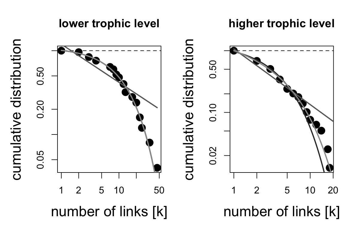
## $`lower level dd fits`
##                         Estimate  Std. Error     Pr(>|t|)        R2       AIC
## exponential          0.082498431 0.002476824 9.830478e-15 0.9970503 -68.92055
## power law            0.455391062 0.055567751 1.033153e-06 0.9226974 -16.52451
## truncated power law -0.001599385 0.031197544 9.598926e-01 0.9970531 -66.92373
##
## $`higher level dd fits`
##                      Estimate Std. Error     Pr(>|t|)        R2       AIC
## exponential         0.3160055 0.01316529 1.641891e-11 0.9966307 -56.23056
## power law           0.9017088 0.06389974 7.797697e-09 0.9794204 -33.33749
## truncated power law 0.2867555 0.05780953 4.285495e-04 0.9984914 -68.93422
3. Network projections
Many network metrics are only available for unipartite networks. One common strategy is to “project” a bipartite to an unipartite network. In its simplest form projecting is done by connecting a pair of nodes in set A of the bipartite network if they are both connected to at least one node in set B. An intuitive way to weigh the edges is by counting the number of nodes in B shared by the dyad in A. Let’s try that:
## connectance
##   0.1513924
# Project plants
plants_projected <- tcrossprod(memmott1999>0) # Number of shared pollinators. Note the diagonal
plants_projected[1:5,1:5]## Agrimonium.eupatorium Leontodon.autumnalis Lotus.corniculatus Medicago.lupulina Rubus.fruticosus
## Agrimonium.eupatorium 8 4 0 1 0
## Leontodon.autumnalis 4 13 0 2 1
## Lotus.corniculatus 0 0 2 0 0
## Medicago.lupulina 1 2 0 2 0
## Rubus.fruticosus 0 1 0 0 1diag(plants_projected) <- 0
g <- graph.adjacency(plants_projected, mode = 'undirected', weighted = T)
par(mar=c(0,0,0,0))
plot(g, vertex.size=6, vertex.label=NA,
edge.color='black', edge.width=log(E(g)$weight),
layout=layout.circle)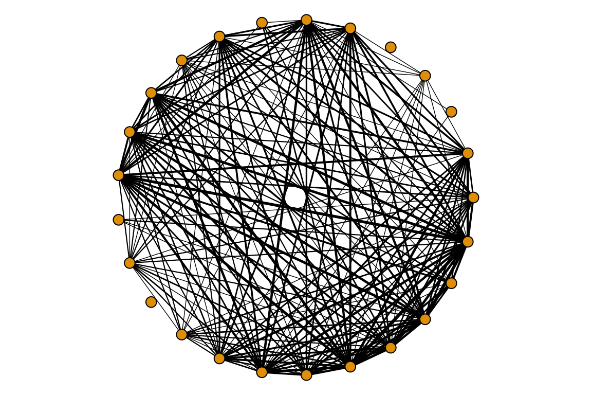
 6. try to project the pollinators
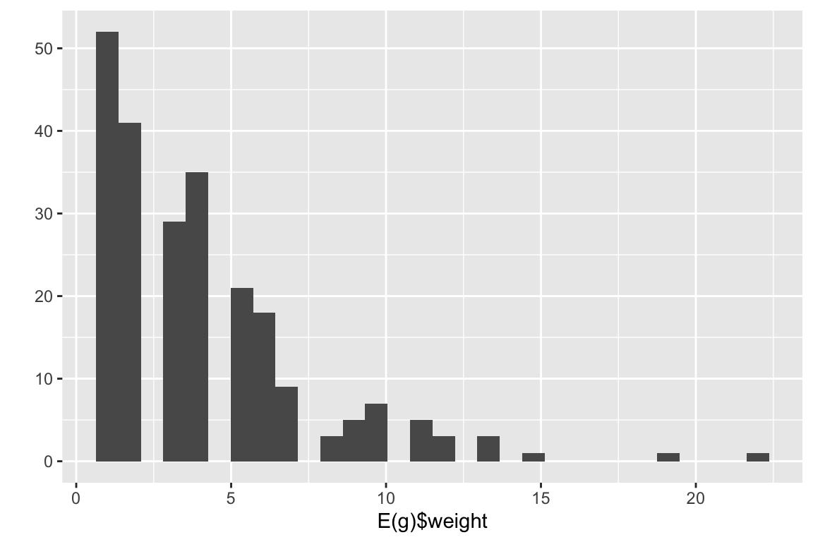
It is also possible to integrate the weights of the edges in the projection. This function in bipartite sums the edge weights of the edges as well.
plants_projected <- as.one.mode(memmott1999, project = 'lower')
g <- graph.adjacency(plants_projected, mode = 'undirected', weighted = T)
qplot(E(g)$weight)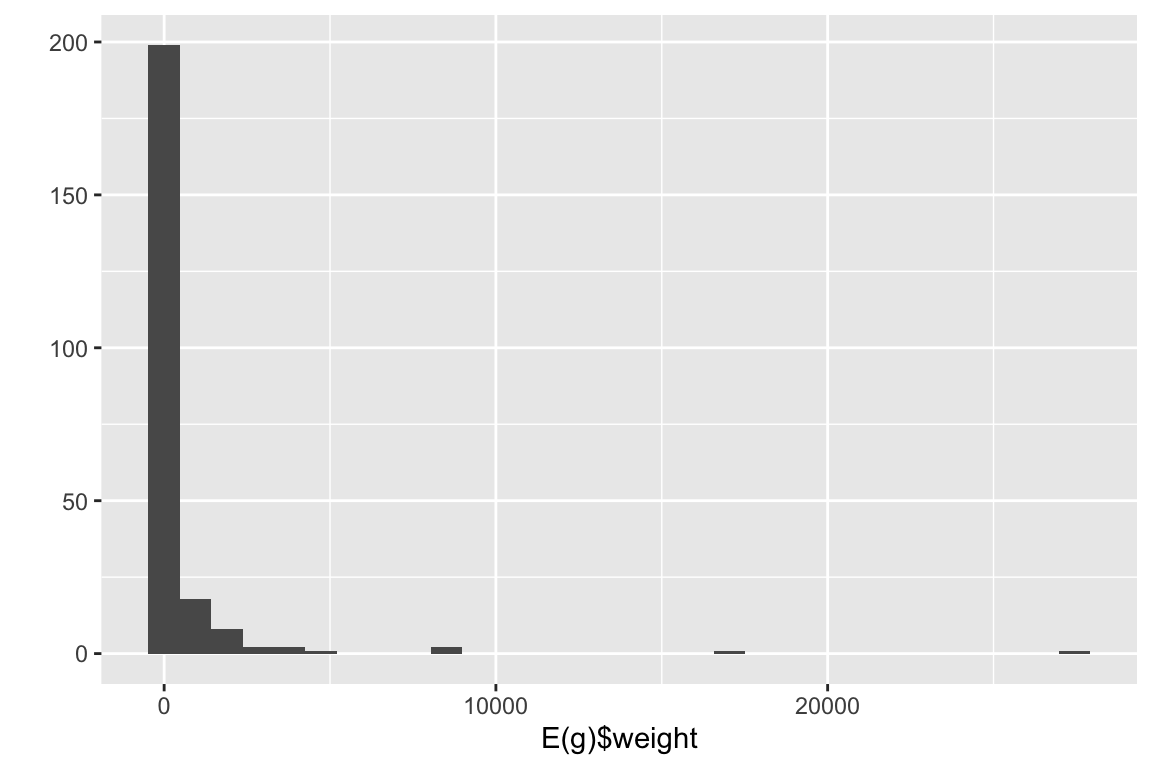
Notice the difference in edge weights.
7. What information do we lose when projecting?
8. What can you say about the density of the projected networks compared to the bipartite version?
9. What is the ecological interpretation of the projections of a plant-pollinator network and of a host-parasite network?
10. Project using a similarity matrix like Jaccard.
4. Unipartite networks
# First, load the data
otago_nodes <- read.csv('data/Otago_Data_Nodes.csv')
otago_links <- read.csv('data/Otago_Data_Links.csv')
otago_web <- graph.data.frame(otago_links, vertices = otago_nodes, directed = T)

# Also load a weighted food web
chesapeake_nodes <- read.csv('data/Chesapeake_bay_nodes.csv', header=F)
names(chesapeake_nodes) <- c('nodeId','species_name')
chesapeake_links <- read.csv('data/Chesapeake_bay_links.csv', header=F)
names(chesapeake_links) <- c('from','to','weight')
ches_web <- graph.data.frame(chesapeake_links, vertices = chesapeake_nodes, directed = T)
# plot(ches_web, edge.width=log(E(ches_web)$weight)/2, layout=layout.circle)
These networks come from the following sources:
- Otago web: Mouritsen KN, Poulin R, McLaughlin JP, Thieltges DW. Food web including metazoan parasites for an intertidal ecosystem in New Zealand. Ecology. Wiley Online Library; 2011;92: 2006–2006., with a description here.
- Chesapeake bay: Baird D, Ulanowicz RE. The Seasonal Dynamics of The Chesapeake Bay Ecosystem. Ecol Monogr. Ecological Society of America; 1989;59: 329–364. Data set is from here
4.1 Degree and strength
The Otago data is unweighted, so we can not calcualte strength. It is
also directed, which means we can separate the in-degree and out-degree.
Let’s take a look at these values. We will use ggplot to
plot the distributions.
deg_dist_out <- igraph::degree(otago_web, mode = 'out')
deg_dist_in <- igraph::degree(otago_web, mode = 'in')
df <- data.frame(deg=c(deg_dist_out,deg_dist_in),
                 direction=c(rep('out',length(deg_dist_in)),rep('in',length(deg_dist_in))))
ggplot(df, aes(deg, fill=direction)) + geom_histogram(alpha=0.3)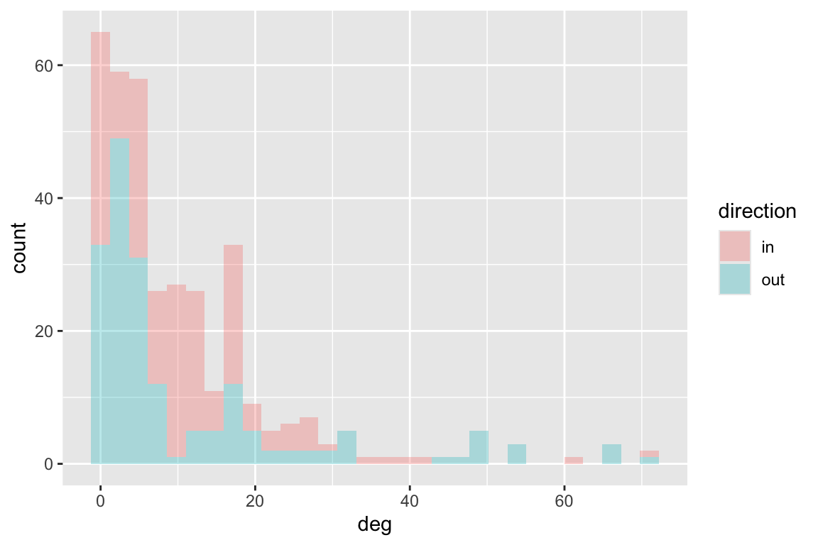
11. Degree (and strength) can be calculated directly from the matrix version of the network. In-degree is \(\sum\limits_{j=1}^J {a_{ij}}\) and out-degree is \(\sum\limits_{i=1}^I {a_{ij}}\). Try to transform the Otago web to an adjacency matrix, then calculate node in-degree and out-degree using the matrix.
The Chesapeake Bay food web is weighted as it describes flow of carbon. So we can calculate degree and strength:
deg_dist_out <- igraph::degree(ches_web, mode = 'out')
deg_dist_in <- igraph::degree(ches_web, mode = 'in')
df <- data.frame(deg=c(deg_dist_out,deg_dist_in),
                 direction=c(rep('out',length(deg_dist_in)),rep('in',length(deg_dist_in))))
ggplot(df, aes(deg, fill=direction))+geom_histogram(alpha=0.3)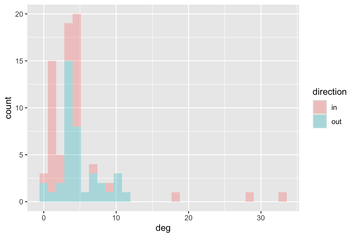
s_dist_out <- igraph::strength(ches_web, mode = 'out')
s_dist_in <- igraph::strength(ches_web, mode = 'in')
df <- data.frame(s=c(s_dist_out,s_dist_in),
                 direction=c(rep('out',length(s_dist_in)),rep('in',length(s_dist_in))))
ggplot(df, aes(s, fill=direction))+geom_histogram(alpha=0.3)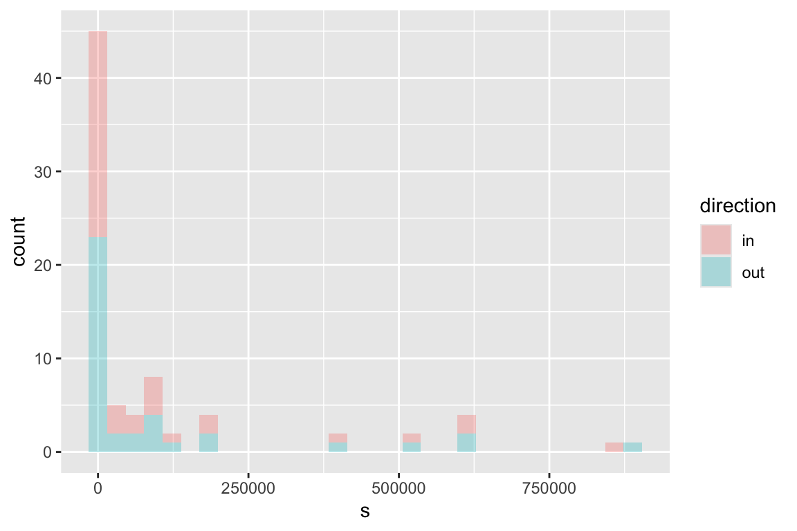
12. Can discrepancies in in-degree and out-degree (or strength) give us some ecological insight?
4.2 Clustering coefficient
The clustering coefficient is a measure of local clustering in a network. It can be defined either locally, per node (number of triangles divided by number of triples), or globally.
# The ratio of the triangles connected to the vertex and the triples centered on the vertex.
transitivity(otago_web, type = 'local')
## 1 2 3 4 5 6 7 8 9 10 11
## 0.20952381 0.09068323 0.21739130 0.36029412 0.20736842 0.09360127 0.10195035 0.20588235 0.26315789 0.26315789 0.10256410
## 12 13 14 15 16 17 18 19 20 21 22
## 0.30882353 0.30882353 0.00000000 0.13333333 0.38333333 0.20512821 0.20512821 0.40672269 0.58479532 0.58479532 0.23894558
## 23 24 25 26 27 28 29 30 31 32 33
## 0.43939394 0.21428571 0.21428571 0.21428571 0.00000000 0.38181818 0.21428571 0.34640523 0.34640523 0.19780220 0.34834835
## 34 35 36 37 38 39 40 41 42 43 44
## 0.34834835 0.34834835 0.32275132 0.30344828 0.28225806 0.00000000 0.27000000 0.27142857 0.17837838 0.17837838 0.40000000
## 45 46 47 48 49 50 51 52 53 54 55
## 0.42105263 0.51052632 0.20000000 0.50724638 0.38461538 0.33333333 0.24264706 0.46825397 0.33333333 0.33333333 0.00000000
## 56 57 58 59 60 61 62 63 64 65 66
## 0.22500000 0.00000000 0.00000000 0.00000000 0.26315789 0.31428571 0.11764706 0.10256410 0.20000000 0.24242424 0.15238095
## 67 68 69 70 71 72 73 74 75 76 77
## 0.21718931 0.24242424 0.30924370 0.27807487 0.40672269 0.24242424 0.60000000 0.22480620 0.22318841 0.50000000 0.39743590
## 78 79 80 81 82 83 84 85 86 87 88
## 0.13888889 0.17948718 0.17948718 0.20000000 0.48421053 0.40000000 0.21052632 0.21052632 0.42365591 0.31159420 0.18947368
## 89 90 91 92 93 94 95 96 97 98 99
## 0.24367816 0.24367816 0.16684685 0.73333333 0.35555556 0.55411255 0.55411255 0.60000000 0.40000000 0.40000000 0.00000000
## 100 101 102 103 104 105 106 107 108 109 110
## 0.12121212 0.32967033 0.13269231 0.38095238 0.38095238 0.28138528 0.29059829 0.14415584 0.11158117 0.24264706 0.13333333
## 111 112 113 114 115 116 117 118 119 120 121
## 0.11168831 0.17094017 0.20000000 0.06926407 0.25000000 0.10039216 0.15019763 0.04736842 0.10114943 0.33333333 0.00000000
## 122 123 124 125 126 127 128 129 130 131 132
## 0.19762846 0.19762846 0.00000000 0.60256410 0.70000000 0.32007401 0.00000000 0.60256410 0.22539683 0.44444444 0.00000000
## 133 134 135 136 137 138 139 140 141 142 143
## 0.60256410 0.70000000 0.34743590 0.00000000 0.70476190 0.70000000 0.27472527 0.00000000 0.60256410 0.46666667 0.44736842
## 144 145 146 147 148 149 150 151 152 153 154
## 0.00000000 0.69166667 0.70000000 0.34502924 0.00000000 0.80555556 0.46666667 0.48538012 0.00000000 0.69166667 0.46666667
## 155 156 157 158 159 160 161 162 163 164 165
## 0.48538012 0.00000000 0.39743590 0.70000000 0.48538012 0.27472527 0.50000000 0.70000000 0.00000000 0.16666667 0.44444444
## 166 167 168 169 170 171 172 173 174 175 176
## 0.00000000 0.49673203 0.00000000 0.49673203 0.25000000 0.48366013 0.31818182 NaN 0.48538012 0.70000000 0.00000000
## 177 178 179 180
## 0.80000000 0.66666667 0.27472527 0.16483516# The ratio of the triangles and the connected triples in the graph
transitivity(otago_web, type = 'global') ## [1] 0.220351213. What can a high local clustering coefficient indicate in a food web?
14. Find another uniparitie network and calculate clusteirng coefficient. Interpret the results.
4.4 Node centrality
There are many centrality metrics, each with dozens of variations. Let’s take a look at the few common ones. Note that it is common to normalize the centrality measures. This is particularly helpful when comparing across networks.
# Assume undirected networks
CC <- igraph::closeness(otago_web, mode = 'all', normalized = T)
BC <- igraph::betweenness(otago_web, directed = F, normalized = T)
EC <- igraph::eigen_centrality(otago_web, directed = F, scale = T)
EC <- EC$vector

# Plot the web, re-sizing nodes by centrality.
V(otago_web)$BC <- BC
par(mar=c(0,0,0,0))
plot(otago_web, vertex.size=BC*100, vertex.label=NA,
     edge.arrow.width=0.5, edge.arrow.size=0.5, edge.curved=0.5,
     layout=layout.circle)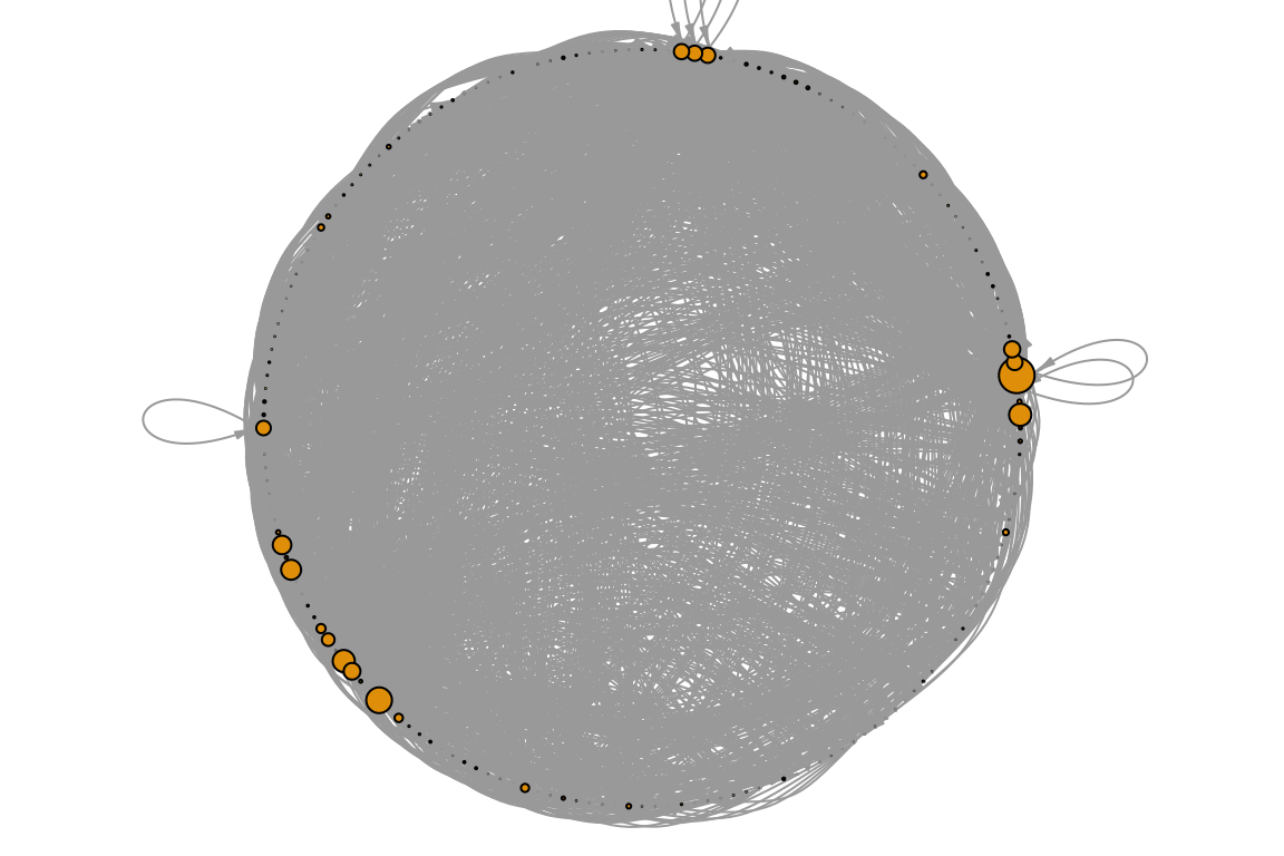
16. Otago is directed so our last calculation was wrong. Calculate the centrality measures for directed food webs.
17. Calculate centrality in your network and interpret the results.
18. What do you think would be the correlation beween these centrality measures? Test it!
19. Which are the most central nodes in your network? Do they have anything in common?
4.4 Motifs and n-node sub-graphs
These are sub-structural patterns composing a network, typically only
meaningful in directed networks. There are 16 kinds of 3-node subgraphs.
See them by calling help: ?triad.census. Let’s plot
them.
par(mfrow=c(4,4), mar=c(.75,.75,.75,.75))
for (i in 0:15){ # note that counting starts at 0
  plot(graph_from_isomorphism_class(size = 3, number = i),
       edge.arrow.size = 0.4,
       edge.color='black',
       main = i + 1)
  box(col='red')
}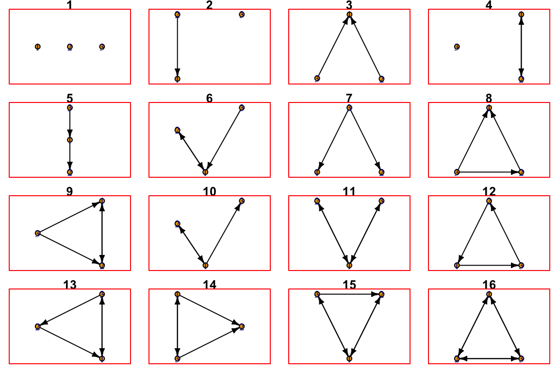
Each of these different classes of subgraphs can have an ecological meaning. For example, #3 means that two prey share a predator and #5 is a trophic chain. It is therefor insightful to quantify how many of each kind are in the food web.
## [1] NA NA 12506 NA 10956 491 22120 3434 533 2287 117 18 57 376 100 49## [1] NA NA 0.2357665334 NA 0.2065455094 0.0092564663 0.4170122917 0.0647387075 0.0100482618
## [10] 0.0431151497 0.0022057160 0.0003393409 0.0010745796 0.0070884549 0.0018852274 0.000923761420. What is the dominant sub-graph in the Otago food web? What is it’s ecological meaning?
21. Calculate the motif profile for another data set. What do the results mean?
5. Advanced exercise: network comparisons
Calculate 10 or more metrics for two or more networks. Use the metrics to compare the networks. You can use, for example ordination analysis. If you do not have data, it is possible to generate random networks in igraph. You can, for example, generate 100 ER networks, 100 scale-free networks and see if they are distinguishable..