Code

Download R code

library(bipartite) # will also load vegan
library(tidyverse)
library(infomapecology)

1. Randomizations for binary matrices

Explanation on the board: why shuffle, algorithms, p-value calculations

We are going to focus on the randomizations of binary bipartite networks, although of course it is possible to randomize unipartite networks (adjacency matrices) and weighted uni/bipartite networks. Randomizations do not generate new data per se, but rather create some randomness through shuffling, in already existing data. The literature on matrix randomizations in Ecology is vast and a few good places to start are specified below in references.

As a general guideline, Here three basic considerations when selecting a randomization procedure:

What is the null hypothesis? For example, randomizing a plant-pollinator matrix while maintaining only the density assumes that pollinators have no dietary restrictions and that plants have not evolved to be specialized for specific pollinators. In other words, that the niche breadth of each species is unlimited in this system. This is obviously a very permissive model.
How sensitive is the model to type-I/II errors
Limitations such as consistency of results and computation time.

In this lab we will see a few algorithms for the sake of introduction. Broadly speaking, in the network ecology literature null models are:

equiprobable: assign the same probability to each potential interaction in the network.
probabilistic: assign a probability to each potential interaction proportional to the number of observed interactions between partners.
fixed: randomly shuffle the interactions while preserving the observed number of partners of each species.

In R, these three kinds of shuffling algorithms are available within vegan. Let’s see them:

library(vegan)
?commsim

1.1 Examples of shuffling

Now let’s shuffle a matrix:

num_iterations <- 10
memmott1999_binary <- 1*(memmott1999>0) # Make the data binary
# Select a null model for the data
null_model <- vegan::nullmodel(memmott1999_binary, method = 'r00') 
shuffled_r00 <- simulate(null_model, nsim = num_iterations) # Shuffle
# Shuffling produces an array with 10 matrices, each of them is a shuffled matrix:
apply(shuffled_r00, 3, dim)

##      sim_1 sim_2 sim_3 sim_4 sim_5 sim_6 sim_7 sim_8 sim_9 sim_10
## [1,]    25    25    25    25    25    25    25    25    25     25
## [2,]    79    79    79    79    79    79    79    79    79     79

#Get shuffled matrix number 10
s10 <- shuffled_r00[,,10]
s10[1:3,1:3]

##                       Coleoptera.spec1 Coleoptera.spec2 Coleoptera.spec3
## Agrimonium.eupatorium                0                0                0
## Leontodon.autumnalis                 0                1                0
## Lotus.corniculatus                   0                0                0

# Calculate the density of each of these matrices:
connectance <- function(m){
  d <- sum(m>0)/(nrow(m)*ncol(m))
  return(d)
}
# Is connectance preserved?:
# Apply the function to the array. Note the MARGIN argument
apply(shuffled_r00, MARGIN = 3, connectance)

##     sim_1     sim_2     sim_3     sim_4     sim_5     sim_6     sim_7     sim_8 
## 0.1513924 0.1513924 0.1513924 0.1513924 0.1513924 0.1513924 0.1513924 0.1513924 
##     sim_9    sim_10 
## 0.1513924 0.1513924

1. What kind of model (equiprobable, probabilistic, fixed) is r00?

2. Can you program the algorithm for r00 by yourself?

r00 does not preserve row or column marginal sums. A more conservative null hypothesis is to conserve either, or both (‘fixed’ null model). Algorithms that conserve both are very restrictive, and are commonly based on randomly selecting 2x2 sub-matrices and then swap their cell entries (“swap” algorithms). However, swap algorithms suffer from several disadvantages in computation time and sampling limitations of the “null space” (discussed in the references below). A new algorithm that overcomes those limitations is the curve ball algorithm (Strona et al. 2014). Note that this is a sequential algorithm in which matrices are generated based on previous ones so for accuracy the first generated matrices should be discarded. This is done using the burnin argument.

num_iterations <- 10
null_model_curveball <- vegan::nullmodel(memmott1999_binary, method = 'curveball') # Select a null model
shuffled_curveball <- simulate(null_model_curveball, nsim = num_iterations, burnin = 1000) #Shuffle
# Calculate the density of each of these matrices
apply(shuffled_curveball, MARGIN = 3, connectance)

##     sim_1     sim_2     sim_3     sim_4     sim_5     sim_6     sim_7     sim_8 
## 0.1513924 0.1513924 0.1513924 0.1513924 0.1513924 0.1513924 0.1513924 0.1513924 
##     sim_9    sim_10 
## 0.1513924 0.1513924

# Did the algorithm match the row and column sums?
all(apply(shuffled_curveball, MARGIN = 3, rowSums)==rowSums(memmott1999_binary)) # all: Are all values true?

## [1] TRUE

all(apply(shuffled_curveball, MARGIN = 3, colSums)==colSums(memmott1999_binary))

## [1] TRUE

# Did it shuffle any interactions?
for (i in 1:num_iterations){
  if(!identical(shuffled_curveball[,,i], memmott1999_binary)){ # If the shuffled is NOT identical to the original
    print(paste('Shuffled matrix',i,'is different than the original'))
  }
}

## [1] "Shuffled matrix 1 is different than the original"
## [1] "Shuffled matrix 2 is different than the original"
## [1] "Shuffled matrix 3 is different than the original"
## [1] "Shuffled matrix 4 is different than the original"
## [1] "Shuffled matrix 5 is different than the original"
## [1] "Shuffled matrix 6 is different than the original"
## [1] "Shuffled matrix 7 is different than the original"
## [1] "Shuffled matrix 8 is different than the original"
## [1] "Shuffled matrix 9 is different than the original"
## [1] "Shuffled matrix 10 is different than the original"

3. There is no better way to understand the mechanics of randomization algorithms than to program one for yourself! Try to program the probabilistic model from [6]: “The probability of each cell being occupied is the average of the probabilities of occupancy of its row and column.” This means that the probability of drawing an interaction is proportional to the degree of both the lower-level and the higher-level species. Mathematically: \(P_{ij}=\left(\frac{\sum A_{i}}{J}+\frac{\sum A_{j}}{I}\right)/2\), where \(A_{ij}\) is the incidence matrix in which \(I\) and \(J\) denote the total number of species in the rows and columns, respectively. Try to program that algorithm. Can you note one problem that you are facing?

1.2 Evaluating significance of Newman’s \(Q\)

Using these randomizations, let’s test if the binary version of the memmot1999 data is “statistically significantly” modular. Here we only present the code, without evaluating it because it takes a lot of time…

web <- memmott1999_binary
mod_observed <- computeModules(web)
Q_obs <- mod_observed@likelihood # This is the value of the modularity function Q for the observed network.

# Now shuffle
num_iterations <- 100
null_model <- vegan::nullmodel(web, method = 'r00') # Only preserve matrix fill (density)
shuffled_r00 <- simulate(null_model, nsim = num_iterations)
# Calculate modularity of the shuffled networks. For each shuffled network store the results in a vector
Q_shuff <- NULL
for (i in 1:100){
  mod <- computeModules(shuffled_r00[,,i])
  Q_shuff <- c(Q_shuff, mod@likelihood)
} 

#Which proportion of the simulations have a Q value larger than the observed?
P_value <- sum(Q_obs < Q_shuff)/length(Q_shuff)

4. Pick another data set from the bipartite package and test if it is significantly modular compared to two null models. Don’t forget to transform it to its binary version! (Or, alternatively, use null models for quantitative networks).

1.3 Evaluating significance of the map equation’s \(L\)

Reminder how to run Infomap:

data(memmott1999)
memmott1999_monolayer_object <- create_monolayer_network(memmott1999_binary,
                                                        bipartite = T, 
                                                        directed = F, 
                                                        group_names = c('Pollinator','Plant'))

## [1] "Input: a bipartite matrix"

memmott1999_monolayer_object$L # The objective function's value

## NULL

Create 500 shuffled matrices of memmott1999_binary. Run infomap on each of the 500 matrices and obtain the 50 \(L\) values. Compare the shuffled values to the observed \(L\): Plot a histogram with the shuffled values and add a vertical line for the observed value. Where does it fall? Calculate the p-value. Is the p-value calculated in the same way as for \(Q\)?

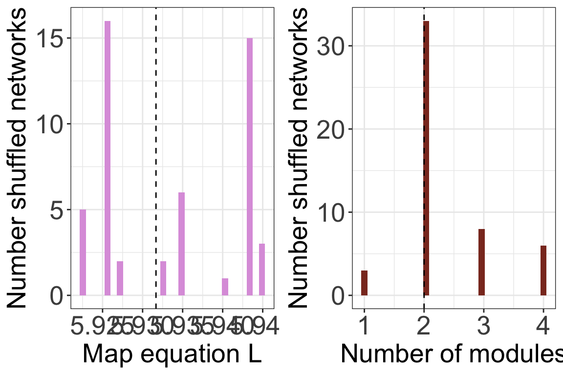
Repeat the previous exercise with the curve ball algorithm. Do the results change?

1.4 Built-in shuffling with infomapecology

The function run_infomap_monolayer can use shuffling algorithms built into vegan. To use this, we need to set signif=T and provide a shuffling method to shuff_method. The shuffling methods are the ones detailed in ?vegan::commsim.

infomap_object <- run_infomap_monolayer(memmott1999_monolayer_object, infomap_executable='./Infomap',
                                        flow_model = 'undirected',
                                        silent=T, trials=20, two_level=T, seed=123,
                                        signif = T, shuff_method = 'r00', nsim = 50)

## [1] "Creating a link list..."
## running: ././Infomap infomap.txt . --tree --seed 123 -N 20 -f undirected --silent --two-level
## [1] "Shuffling..."
## [1] "Running Infomap on shuffled network 1/50"
## [1] "Running Infomap on shuffled network 2/50"
## [1] "Running Infomap on shuffled network 3/50"
## [1] "Running Infomap on shuffled network 4/50"
## [1] "Running Infomap on shuffled network 5/50"
## [1] "Running Infomap on shuffled network 6/50"
## [1] "Running Infomap on shuffled network 7/50"
## [1] "Running Infomap on shuffled network 8/50"
## [1] "Running Infomap on shuffled network 9/50"
## [1] "Running Infomap on shuffled network 10/50"
## [1] "Running Infomap on shuffled network 11/50"
## [1] "Running Infomap on shuffled network 12/50"
## [1] "Running Infomap on shuffled network 13/50"
## [1] "Running Infomap on shuffled network 14/50"
## [1] "Running Infomap on shuffled network 15/50"
## [1] "Running Infomap on shuffled network 16/50"
## [1] "Running Infomap on shuffled network 17/50"
## [1] "Running Infomap on shuffled network 18/50"
## [1] "Running Infomap on shuffled network 19/50"
## [1] "Running Infomap on shuffled network 20/50"
## [1] "Running Infomap on shuffled network 21/50"
## [1] "Running Infomap on shuffled network 22/50"
## [1] "Running Infomap on shuffled network 23/50"
## [1] "Running Infomap on shuffled network 24/50"
## [1] "Running Infomap on shuffled network 25/50"
## [1] "Running Infomap on shuffled network 26/50"
## [1] "Running Infomap on shuffled network 27/50"
## [1] "Running Infomap on shuffled network 28/50"
## [1] "Running Infomap on shuffled network 29/50"
## [1] "Running Infomap on shuffled network 30/50"
## [1] "Running Infomap on shuffled network 31/50"
## [1] "Running Infomap on shuffled network 32/50"
## [1] "Running Infomap on shuffled network 33/50"
## [1] "Running Infomap on shuffled network 34/50"
## [1] "Running Infomap on shuffled network 35/50"
## [1] "Running Infomap on shuffled network 36/50"
## [1] "Running Infomap on shuffled network 37/50"
## [1] "Running Infomap on shuffled network 38/50"
## [1] "Running Infomap on shuffled network 39/50"
## [1] "Running Infomap on shuffled network 40/50"
## [1] "Running Infomap on shuffled network 41/50"
## [1] "Running Infomap on shuffled network 42/50"
## [1] "Running Infomap on shuffled network 43/50"
## [1] "Running Infomap on shuffled network 44/50"
## [1] "Running Infomap on shuffled network 45/50"
## [1] "Running Infomap on shuffled network 46/50"
## [1] "Running Infomap on shuffled network 47/50"
## [1] "Running Infomap on shuffled network 48/50"
## [1] "Running Infomap on shuffled network 49/50"
## [1] "Running Infomap on shuffled network 50/50"

## [1] "Removing auxilary files..."

# Plot histograms
plots <- plot_signif(infomap_object, plotit = F)
plot_grid(
  plots$L_plot+
    theme_bw()+
    theme(legend.position='none',
          axis.text = element_text(size=20),
          axis.title = element_text(size=20)),
  plots$m_plot+
    theme_bw()+
    theme(legend.position='none',
          axis.text = element_text(size=20),
          axis.title = element_text(size=20))
)

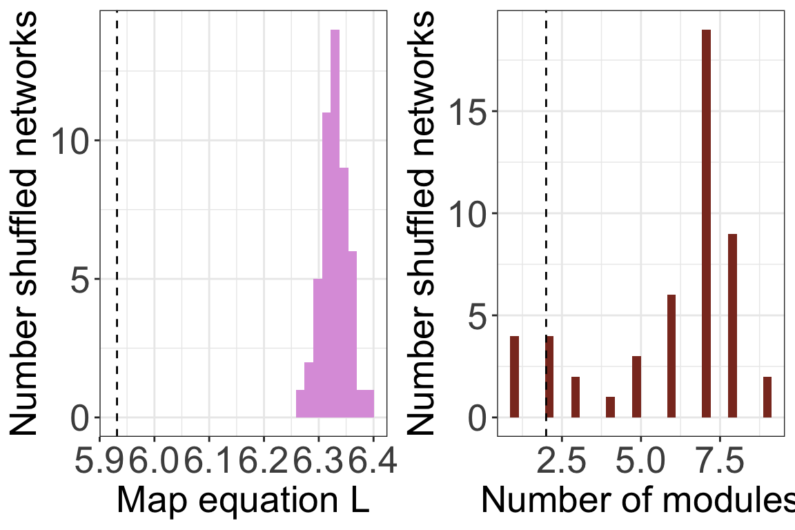
Another way is to provide shuff_method with a list containing already shuffled networks. You can use the function shuffle_infomap to produce shuffled networks with vegan or you can use any other method.

shuffled <- shuffle_infomap(memmott1999_monolayer_object, 
                            shuff_method='curveball', 
                            nsim=50, burnin=2000)

## [1] "Shuffling..."

infomap_object <- run_infomap_monolayer(memmott1999_monolayer_object,
                                        infomap_executable='./Infomap',
                                        flow_model = 'undirected',
                                        silent=T, trials=20, two_level=T, seed=123,
                                        signif = T, shuff_method = shuffled, nsim = 50)

## [1] "Creating a link list..."
## running: ././Infomap infomap.txt . --tree --seed 123 -N 20 -f undirected --silent --two-level
## [1] "Running Infomap on shuffled network 1/50"
## [1] "Running Infomap on shuffled network 2/50"
## [1] "Running Infomap on shuffled network 3/50"
## [1] "Running Infomap on shuffled network 4/50"
## [1] "Running Infomap on shuffled network 5/50"
## [1] "Running Infomap on shuffled network 6/50"
## [1] "Running Infomap on shuffled network 7/50"
## [1] "Running Infomap on shuffled network 8/50"
## [1] "Running Infomap on shuffled network 9/50"
## [1] "Running Infomap on shuffled network 10/50"
## [1] "Running Infomap on shuffled network 11/50"
## [1] "Running Infomap on shuffled network 12/50"
## [1] "Running Infomap on shuffled network 13/50"
## [1] "Running Infomap on shuffled network 14/50"
## [1] "Running Infomap on shuffled network 15/50"
## [1] "Running Infomap on shuffled network 16/50"
## [1] "Running Infomap on shuffled network 17/50"
## [1] "Running Infomap on shuffled network 18/50"
## [1] "Running Infomap on shuffled network 19/50"
## [1] "Running Infomap on shuffled network 20/50"
## [1] "Running Infomap on shuffled network 21/50"
## [1] "Running Infomap on shuffled network 22/50"
## [1] "Running Infomap on shuffled network 23/50"
## [1] "Running Infomap on shuffled network 24/50"
## [1] "Running Infomap on shuffled network 25/50"
## [1] "Running Infomap on shuffled network 26/50"
## [1] "Running Infomap on shuffled network 27/50"
## [1] "Running Infomap on shuffled network 28/50"
## [1] "Running Infomap on shuffled network 29/50"
## [1] "Running Infomap on shuffled network 30/50"
## [1] "Running Infomap on shuffled network 31/50"
## [1] "Running Infomap on shuffled network 32/50"
## [1] "Running Infomap on shuffled network 33/50"
## [1] "Running Infomap on shuffled network 34/50"
## [1] "Running Infomap on shuffled network 35/50"
## [1] "Running Infomap on shuffled network 36/50"
## [1] "Running Infomap on shuffled network 37/50"
## [1] "Running Infomap on shuffled network 38/50"
## [1] "Running Infomap on shuffled network 39/50"
## [1] "Running Infomap on shuffled network 40/50"
## [1] "Running Infomap on shuffled network 41/50"
## [1] "Running Infomap on shuffled network 42/50"
## [1] "Running Infomap on shuffled network 43/50"
## [1] "Running Infomap on shuffled network 44/50"
## [1] "Running Infomap on shuffled network 45/50"
## [1] "Running Infomap on shuffled network 46/50"
## [1] "Running Infomap on shuffled network 47/50"
## [1] "Running Infomap on shuffled network 48/50"
## [1] "Running Infomap on shuffled network 49/50"
## [1] "Running Infomap on shuffled network 50/50"
## [1] "Removing auxilary files..."

plots <- plot_signif(infomap_object, plotit = F)

plot_grid(
  plots$L_plot+
  theme_bw()+
  theme(legend.position='none',
        axis.text = element_text(size=20),
        axis.title = element_text(size=20)),
  plots$m_plot+
    theme_bw()+
    theme(legend.position='none',
          axis.text = element_text(size=20),
          axis.title = element_text(size=20))
)

2. Recommended workflow

The algorithms that calculate modularity and assign species to modules are not deterministic. These are search algorithms that may produce different results each time they are run. In addition, the value of the objective function can only be interpreted in a relation to a null expectation. Therefore, a typical workflow when working with data would be as follows. This example is for \(L\):

Calculate \(L\) for the empirical network multiple (usually 100) times. This can be done with the trials argument in run_infomap_monolayer.
Select the run with \(min(L)\) and use this as the \(L_{obs}\).
Decide on a randomization scheme and produce an ensemble of shuffled networks (usually >=1000).
Calculate the \(L_{null}\) for each of these shuffled networks and create a distribution of these values.
Calculate the P value as the proportion of times \(L_{null}<L_{obs}\).

3. Advanced (but necessary) topics

Hypothesis testing is a whole world. Here we just described the basis. I recommend reading (Gotelli and Ulrich 2012). In that paper they also mention process-based null models, which are a whole different class of concepts and methods. Here are three main topics that you will probably need to go deeper into when you analyze your on data:

Weighted matrices: With weighted matrices the logic and workflow is the same as with binary data but the shuffling methods are different. Some shuffling algorithms work similarly to binary matrices: they conserve for example row or column sums. Others shuffle the underlying binary structure and redistribute the weights see (Ulrich and Gotelli 2010) and ?commsim for details.
Neutral models: Shuffling as-is does not take into account neutral processes. It may also be necessary to include aspects like abundance because the interactions between speceis can be a result of abundance rather than a true interaction.
Z-scores: Many studies use z-scores to compare shuffled and observed data. It is worthwhile understanding this method, and its limitations. See (Song et al. 2017) and (Song et al. 2019).
Methods: A new package to analyze null model is econullnetr (Vaughan et al. 2018).

References

Gotelli, Nicholas J, and Werner Ulrich. 2012. “Statistical Challenges in Null Model Analysis.” Oikos 121 (February): 171–80. https://doi.org/10.1111/j.1600-0706.2011.20301.x.

Song, Chuliang, Rudolf P Rohr, and Serguei Saavedra. 2017. “Why Are Some Plant–Pollinator Networks More Nested Than Others?” J. Anim. Ecol. 86 (November): 1417–24. https://doi.org/10.1111/1365-2656.12749.

Song, Chuliang, Rudolf P Rohr, and Serguei Saavedra. 2019. “Beware z-Scores.” J. Anim. Ecol. 88 (May): 808–9. https://doi.org/10.1111/1365-2656.12964.

Strona, Giovanni, Domenico Nappo, Francesco Boccacci, Simone Fattorini, and Jesus San-Miguel-Ayanz. 2014. “A Fast and Unbiased Procedure to Randomize Ecological Binary Matrices with Fixed Row and Column Totals.” Nat. Commun. 5 (June): 4114. https://doi.org/10.1038/ncomms5114.

Ulrich, Werner, and Nicholas J Gotelli. 2010. “Null Model Analysis of Species Associations Using Abundance Data.” Ecology 91 (November): 3384–97.

Vaughan, Ian P, Nicholas J Gotelli, Jane Memmott, Caitlin E Pearson, Guy Woodward, and William O C Symondson. 2018. “Econullnetr: An r Package Using Null Models to Analyse the Structure of Ecological Networks and Identify Resource Selection.” Methods Ecol. Evol. 9 (March): 728–33. https://doi.org/10.1111/2041-210x.12907.

Lab: Hypothesis testing

Last update: 03 March, 2026