Lab: Robustness

Code

Download R code

library(bipartite) # will also load vegan
library(tidyverse)
library(vegan)

1. Network robustness

The question of how networks with different structures respond to failure of (or attack on) nodes is fundamental across all of network science. For example, in information security, attack on a hub site vs a random site will result in fundamentally different cascades of information failure. These concepts are naturally adapted in ecology. For example, how will a food web collapse if the most connected species go extinct first, compared to when extinctions are random? In our next exercise we will try to build an algorithm for simulating species extinctions in food webs. 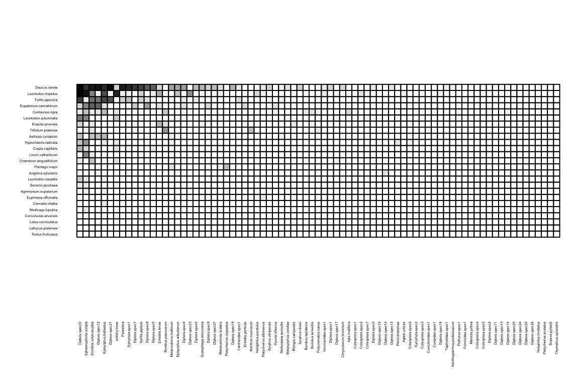Yet to give you a sense of how such analysis can look like, let’s first take a look at existing implementation in R for bipartite networks. In the following implantation we simulate an extinction process of the plants. There are 3 possible scenarios to extinction (Memmott et al. 2004):

1. Least connected –> most connected
2. Most connected –> leaset connected
3. Random

data("memmott1999")
visweb(memmott1999)

# Follow secondary extinction of pollinators, while removing plants.
ex_random <- second.extinct(memmott1999, method = 'random', participant = 'lower', nrep=100, details=F) # Replicate simulations because it is random.
ex_random[1:3,]

##      no ext.lower ext.higher
## [1,]  1         1       1.07
## [2,]  2         1       0.59
## [3,]  3         1       1.17

ex_least <- second.extinct(memmott1999, method = 'abundance', participant = 'lower', details=F)
ex_least[1:3,]

##      no ext.lower ext.higher
## [1,]  1         1          0
## [2,]  2         1          0
## [3,]  3         1          0

ex_most <- second.extinct(memmott1999, method = 'degree', participant = 'lower', details=F)
ex_most[1:3,]

##      no ext.lower ext.higher
## [1,]  1         1         10
## [2,]  2         1          6
## [3,]  3         1          3

We can then plot an Attack Tolerance Curve (Burgos et al. 2007). These plots are built-in and very difficult to tweak directly. The function returns the exponent \(a\) of \(y \sim 1 - x^a\). So \(a\) is a measure of extinction vulnerability. The more gradual the secondary extinctions, the lower the absolute value of \(a\). Or, phrased differently, large absolute values of \(a\) indicate a very abrupt die-off, indicative of high initial redundancy in the network.’’ (from ?slope.bipartite).

par(mfrow=c(2,2))
slope.bipartite(ex_random, cex.axis=0.1) #fit a curve to the extinction data

## exponent 
## 2.488223

slope.bipartite(ex_least) #fit a curve to the extinction data

## exponent 
## 15.26302

slope.bipartite(ex_most) #fit a curve to the extinction data

##  exponent 
## 0.5799287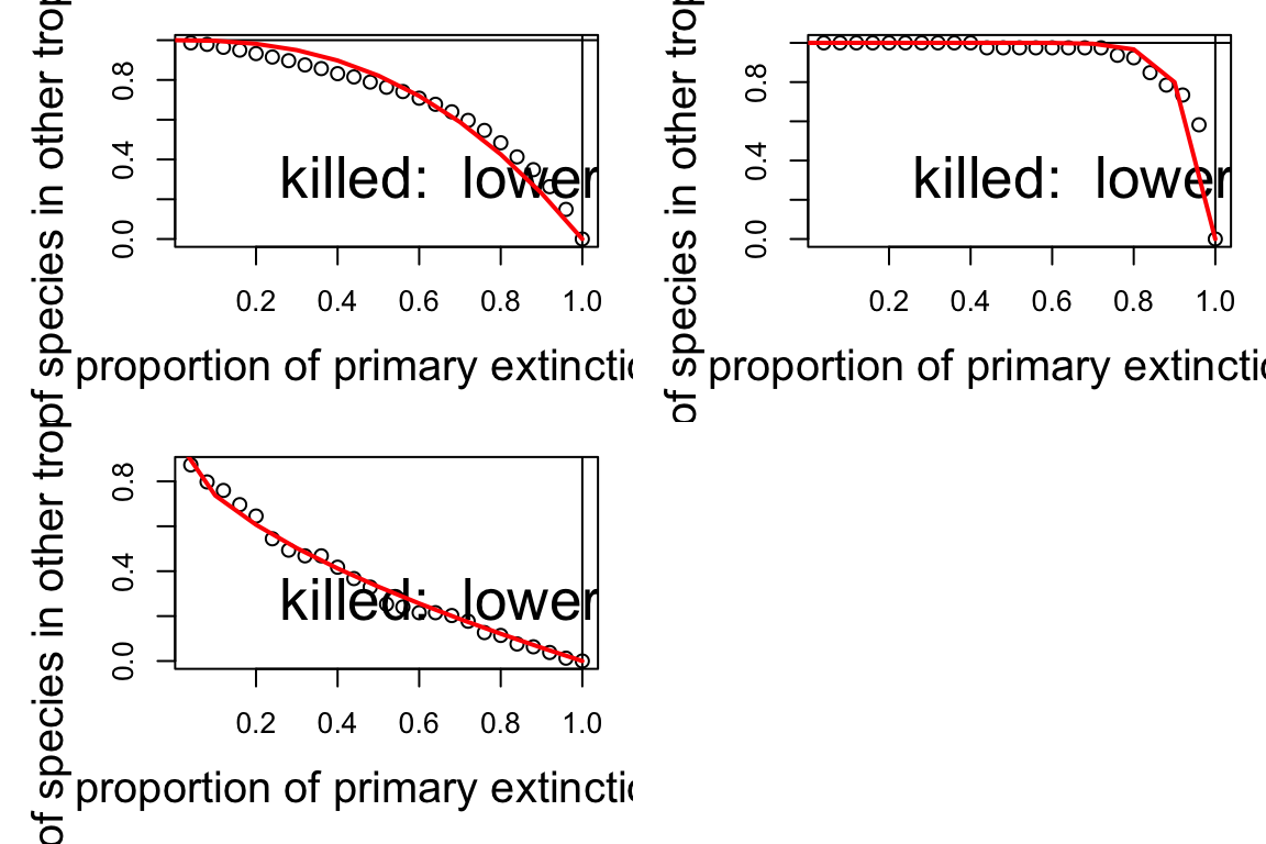

The area under the curve can be used to quantify “robustness”, as suggested (Burgos et al. 2007).

# Robustness
robustness(ex_random)

## [1] 0.665792

robustness(ex_least)

## [1] 0.8873465

robustness(ex_most)

## [1] 0.3259379

What can you say about the tolerance of the network to different extinction regimes?

Repeat that exercise, now removing pollinators. Is the tolerance of the network different?

Advanced exercise: To understand how robustness is affected by network properties, generate an ensemble of networks of different topologies (e.g., size and density), and test their robustness. Can you find any associations between topology and robustness? Specifically, try to test the relationship between nestedness and robustness. Does robustness correlate positively with nestedness? under which regime of extinction?

2. Programming an algorithm for extinction cascades

In this part you will try to program an algorithm for secondary extinctions.

References

Burgos, Enrique, Horacio Ceva, Roberto P J Perazzo, et al. 2007. “Why Nestedness in Mutualistic Networks?” J. Theor. Biol. 249 (November): 307–13. https://doi.org/10.1016/j.jtbi.2007.07.030.

Memmott, Jane, Nickolas M Waser, and Mary V Price. 2004. “Tolerance of Pollination Networks to Species Extinctions.” Proc. R. Soc. B 271 (December): 2605–11. https://doi.org/10.1098/rspb.2004.2909.